Acknowledgements

HEAT crash and carbon modules and updated 2017 version (HEAT 4.0) (2016-2017)

Lead authors

·       Thomas Götschi, University of Zurich, Switzerland

·       Alberto Castro Fernandez, University of Zurich, Switzerland

·       Christian Brand, University of Oxford, United Kingdom

·       James Woodcock, University of Cambridge, United Kingdom

·       Sonja Kahlmeier, University of Zurich, Switzerland

Software development and design

·       Tomasz Szreniawski,

·       Alberto Castro Fernandez,

·       Ali Abbas,

·       Vicki Copley

·       Thomas Götschi

Text editing

·       David Breuer

·       Sonja Kahlmeier

·       Nick Cavill

Project core group

·       Harry Rutter, London School of Hygiene and Tropical Medicine, United Kingdom

·       Francesca Racioppi, WHO Regional Office for Europe

·       Sonja Kahlmeier, University of Zurich, Switzerland

·       Thomas Götschi, University of Zurich, Switzerland

·       Nick Cavill, Cavill Associates, United Kingdom

·       James Woodcock, University of Cambridge, United Kingdom

·       Paul Kelly, University of Edinburgh, United Kingdom

·       Christian Brand, University of Oxford, United Kingdom

·       David Rojas Rueda, Barcelona Institute for Global Health (ISGlobal), Spain

·       Alberto Castro Fernandez, University of Zurich, Switzerland

·       Christoph Lieb/Heini Sommer, Ecoplan, Switzerland

·       Christian Schweizer, WHO Regional Office for Europe

·       Pekka Oja, UKK Institute for Health Promotion Research, Finland

·       Charlie Foster, University of Bristol, United Kingdom

International advisory group

·       Andrew Cope, Sustrans, United Kingdom

·       Bas De Geus, Free University Brussels, Belgium

·       Audrey de Nazelle, Imperial College London, United Kingdom

·       Rune Elvik, Institute of Transport Economics, Norway

·       Frank George, WHO Regional Office for Europe

·       Anna Goodman, London School of Hygiene & Tropical Medicine, United Kingdom

·       Nicole Iroz-Elardo, Urban Design 4 Health, Rochester, United States

·       Thiago Herick de Sa / Meleckidzedeck Khayesi / Pierpaolo Mudu, WHO Headquarters

·       Eva Heinen, University of Leeds, United Kingdom

·       Michal Krzyzanowski, consultant, Poland

·       Pekka Oja, UKK Institute for Health Promotion Research, Finland

·       Randy Rzewnicki, European Cyclists’ Federation, Belgium

·       Alexandre Santacreu, International Transport Forum, France

·       Lucinda Saunders, Greater London Authority/Transport for London, United Kingdom

·       Jan Sorensen, Royal College of Surgeons, Ireland

·       Joe Spadaro, WHO Regional Office for Europe

·       Marko Tainio, University of Cambridge, United Kingdom

·       Miles Tight, University of Birmingham, United Kingdom

·       George Georgiadis / Virginia Fuse, United Nations Economic Commission for Europe

Acknowledgements

The 2017 update of HEAT for cycling and walking was supported in part by the project “Physical Activity through Sustainable Transport Approaches” (PASTA) (http://pastaproject.eu), which is funded by the European Union’s Seventh Framework Program under EC-GA No. 602624-2 (FP7-HEALTH-2013-INNOVATION-1).

The 5^th consensus workshop (28-29 March 2017, Copenhagen, Denmark) was chaired by Michal Krzyzanowski, Poland, and facilitated by the University of Zurich, Switzerland.

Back to homepage         Back to how HEAT works            Back to acknowledgements

Development of the HEAT air pollution module (2014-2015)

Lead authors

·       David Rojas Rueda, Centre  for Research in Environmental Epidemiology, Spain

·       Audrey Nazelle, University College London, United Kingdom

·       Sonja Kahlmeier, University of Zurich, Switzerland

·       Christian Schweizer, WHO Regional Office for Europe

Project core group

·       Harry Rutter, London School of Hygiene and Tropical Medicine, United Kingdom

·       Francesca Racioppi, WHO Regional Office for Europe

·       Sonja Kahlmeier, University of Zurich, Switzerland

·       Christian Schweizer, WHO Regional Office for Europe

·       Nick Cavill, Cavill Associates, United Kingdom

·       Hywell Dinsdale, consultant, United Kingdom

·       Thomas Götschi, University of Zurich, Switzerland

·       James Woodcock, Institute of Public Health, Cambridge, United Kingdom

·       Paul Kelly, Oxford University/University of Edinburgh, United Kingdom

·       Christoph Lieb/Heini Sommer, Ecoplan

·       Pekka Oja, UKK Institute for Health Promotion Research, Finland

·       Charlie Foster, Oxford  University,  United Kingdom

International advisory group

·       Karim Abu-Omar,  University of  Erlangen, Germany

·       Hugh Ross Anderson, St George’s University of London, United Kingdom

·       Olivier Bode, University College London, United Kingdom

·       Tegan Boehmer, Centers for Disease Control and Prevention, United States of America

·       Francesco Forastiere, Azienda Sanitaria Locale RME, Rome, Italy

·       Eszter  Füzeki, Johann  Wolfgang  Goethe-Universität, Germany

·       Gerard Hoek, University of Utrecht, the Netherlands

·       Frank George, WHO Regional Office for Europe

·       Marie-Eve Heroux, WHO Regional Office for Europe

·       Michal Krzyzanowski, King’s College London, United Kingdom

·       Mark Nieuwenhuijsen, Centre  for Research in Environmental Epidemiology, Spain

·       Luc Int Panis, VITO, Belgium

·       Laura Perez, Swiss Tropical and Public Health Institute, Switzerland

·       Marko Tainio, University of Cambridge, United Kingdom

Acknowledgements

The development of the air pollution module of HEAT and the 2015 version of this publication was supported by the German Federal Ministry for the Environment, Nature Conservation, Building and Nuclear Safety. The fourth consensus workshop (Bonn, Germany, 11-12 December 2014) was chaired by Michal Krzyzanowski, King’s College London and facilitated by the University of Zurich,  Switzerland.

Back to homepage         Back to how HEAT works            Back to acknowledgements

Acknowledgements

HEAT for cycling and walking 2014 update

These tools have been developed from an original idea of Harry Rutter, National Obesity Observatory England, United Kingdom and they are based on the principles of the Health Economic Assessment Tool for Cycling first published in 2007.

Project core group

·       Sonja Kahlmeier, University of Zurich, Switzerland

·       Paul Kelly, University of Oxford, United Kingdom

·       Charlie Foster, University of Oxford, United Kingdom

·       Thomas Götschi, University of Zurich, Switzerland

·       Nick Cavill, Cavill Associates, United Kingdom

·       Hywell Dinsdale, Public Health Analyst, Hyde, United Kingdom

·       James Woodcock, University of Cambridge, United Kingdom

·       Christian Schweizer, WHO Regional Office for Europe

·       Harry Rutter, London School of Hygiene and Tropical Medicine, United Kingdom

·       Christoph Lieb, Ecoplan, Switzerland

·       Pekka Oja, UKK Institute for Health Promotion Research, Finland

·       Francesca Racioppi, WHO Regional Office for Europe

Web programming and design:

·       Duy Dao, Switzerland

Text editing:

·       Nicoletta di Tanno,

·       Sonja Kahlmeier,

·       Nick Cavill,

·       Christian Schweizer

International advisory group

·       Karim Abu-Omar, University Erlangen, Germany

·       Lars Bo Andersen, School of Sports Science, Norway

·       Finn Berggren, Gerlev Physical Education and Sports Academy, Denmark

·       Tegan Boehmer, Centers for Disease Control and Prevention, USA

·       Nils-Axel Braathen, Organization for Economic Cooperation and Development (OECD), France

·       Audrey de Nazelle, University College London, United Kingdom

·       Jonas Finger, Robert Koch Institute, Germany

·       I-Min Lee, Harvard School of Public Health, USA

·       Eszter Füzeki, Johann Wolfgang Goethe-Universität, Germany

·       Frank George, Health Economics , WHO Regional Office for Europe

·       Regine Gerike, University of Natural Resources and Life Sciences Vienna, Austria

·       Marie-Eve Heroux, Air Quality, WHO Regional Office for Europe

·       Michal Krzyzanowski, King's College London, United Kingdom

·       Nanette Mutrie, University of Edinburgh, United Kingdom

·       Peter Schantz,The Swedish School of Sport and Health Sciences, Sweden

·       Luc Int Panis, VITO, Belgium

·       Laura Perez, Swiss Tropical and Public Health Institute, Switzerland

·       Heini Sommer, Ecoplan, Switzerland

·       David Rojas Rueda, Centre for Research in Environmental Epidemiology (CREAL), Spain

Acknowledgements

This 2014 update of HEAT for cycling and walking was supported by the German Federal Ministry for the Environment, Nature Conservation, Building and Nuclear Safety. The third consensus workshop (Bonn, Germany, 1-2 October 2013) was chaired by Michal Krzyzanowski, King’s College London, facilitated by the University of Zurich, Switzerland, and carried out in collaboration with the Universitätsclub Bonn e.V.

We wish to thank Nia Roberts, Peter Scarborough, Justin Richards, Andrew Wright, Aiden Doherty and Anja Mizdrak, Oxford University, for their contributions to the systematic reviews on cycling and walking and all-cause mortality and Dareskedar Workie, University of Alberta, Canada, for input to the economic valuation approach.

Back to homepage         Back to how HEAT works            Back to acknowledgements

Acknowledgements

Health Economic Assessment Tool for walking (2010-2011)

This tool has been developed from an original idea of Harry Rutter, National Obesity Observatory England, United Kingdom and it is based on the principles of the Health Economic Assessment Tool for Cycling first published in 2007.

Lead authors

·       Hywell Dinsdale, National Obesity Observatory England, United Kingdom (Tool programming and technical development)

·       Nick Cavill, Cavill Associates, United Kingdom (Project management and technical development)

·       Sonja Kahlmeier, University of Zurich, Switzerland (Project management and technical development)

Project core group

·       Sonja Kahlmeier, University of Zurich, Switzerland

·       Nick Cavill, Cavill Associates, United Kingdom

·       Hywell Dinsdale, National Obesity Observatory England, United Kingdom

·       Harry Rutter, National Obesity Observatory England, United Kingdom

·       Thomas Götschi, University of Zurich, Switzerland

·       Charlie Foster, University of Oxford, United Kingdom

·       Paul Kelly, University of Oxford, United Kingdom

·       Dushy Clarke, University of Oxford, United Kingdom

·       Pekka Oja, UKK Institute for Health Promotion Research, Finland

·       Richard Fordham, University of East Anglia, United Kingdom

·       Dave Stone, Natural England, United Kingdom

·       Francesca Racioppi, WHO European Centre for Environment and Health, Rome, WHO Regional Office for Europe

Web programming and design:

·       Duy Dao, Switzerland

Text editing:

·       Nicoletta di Tanno

·       Sonja Kahlmeier

·       Nick Cavill

International advisory group

Pilot testing:

·       Hana Bruhova-Foltynova, Charles University Environment Centre, Czech Republic

·       Sean Co, Metropolitan Transportation Commission, Oakland, California, United States of America

·       Werner Hagens, Liesbeth Mathijssen, Yonne Mulder, National Institute for Public Health and the Environment (RIVM), the Netherlands

·       Ruth Hunter, Centre for Public Health, Queen's University Belfast, United Kingdom

·       Sam Margolis, LBTH and NHS Tower Hamlets, United Kingdom

·       Angela Wilson, Research and Monitoring Unit, Sustrans, United Kingdom

The project was supported by a consortium of donors from the United Kingdom under the leadership of Natural England. The consortium included the Department of Health England, Environment Agency, Countryside Council for Wales, Public Health Wales, Physical Activity & Nutrition Networks for Wales, Forestry Commission and the Scottish Government, Public Health Directorate. It was also supported by the Swiss Federal Office of Public Health and by the WHO Regional Office of Europe.

It was carried out in close collaboration with HEPA Europe, the European network for the promotion of health-enhancing physical activity, and the Transport, Health and Environment Pan-European Programme (THE PEP). The consensus workshop (Oxford, United Kingdom, 1-2 July 2010) was facilitated by the University of Oxford.

The development of HEAT Walking was also financially supported by the European Union in the framework of the Health Programme 2008-2013 (Grant agreement 2009 52 02). The views expressed herein can in no way be taken to reflect the official opinion of the European Union.

Back to homepage         Back to how HEAT works            Back to acknowledgements

Acknowledgements

Health Economic Assessment Tool for cycling (2007-2010)

This tool has been developed by:

·       Harry Rutter, South East Public Health Observatory, United Kingdom

·       Nick Cavill, Cavill Associates, United Kingdom

·       Hywell Dinsdale, South East Public Health Observatory, United Kingdom

·       Sonja Kahlmeier, WHO European Centre for Environment and Health, Rome, WHO Regional Office for Europe

·       Francesca Racioppi, WHO European Centre for Environment and Health, Rome, WHO Regional Office for Europe

·       Pekka Oja, Karolinska Institute, Sweden

Web programming and design:

·       Duy Dao, Switzerland

Text editing:

·       Nicoletta di Tanno

·       Sonja Kahlmeier

·       Nick Cavill

An international advisory group contributed to the development of this tool:

 * members of the extended core group

Pilot testing:

·       Hana Bruhova-Foltynova, Charles University Environment Centre, Czech Republic

·       Sean Co, Metropolitan Transportation Commission, Oakland, California, United States of America

·       Werner Hagens, Liesbeth Mathijssen, Yonne Mulder, National Institute for Public Health and the Environment (RIVM), the Netherlands

·       Ruth Hunter, Centre for Public Health, Queen's University Belfast, United Kingdom

·       Sam Margolis, LBTH and NHS Tower Hamlets, United Kingdom

·       Angela Wilson, Research and Monitoring Unit, Sustrans, United Kingdom

The project was supported by the Austrian Federal Ministry of Agriculture, Forestry, Environment and Water Management, Division V/5 – Transport, Mobility, Human Settlement and Noise and by the Swedish Expertise Fund, and facilitated by the Karolinska Institute, Sweden. The project benefited greatly from systematic reviews being undertaken for the National Institute for Health and Clinical Excellence (NICE) in the United Kingdom. The consensus workshop (Graz, Austria, 15–16 May 2007) was facilitated by the University of Graz.

The update of HEAT Cycling in 2011 was also financially supported by the European Union in the framework of the Health Programme 2008-2013 (Grant agreement 2009 52 02). The views expressed herein can in no way be taken to reflect the official opinion of the European Union.

Back to homepage         Back to how HEAT works            Back to acknowledgements

How to navigate the tool

Depending on the characteristics of an assessment, a varying number of questions will apply to a specific HEAT assessment. A maximum of 21 questions will be asked; depending on the route you take, you will skip some questions. On the left side of the screen, the menu of pages helps you to orient yourself on where you are in the assessment process.

Click on “next” or “back” to move between pages. You can also go back to a previous question to check or change entries by clicking on the section in the menu to which this question belongs (see also below) in the menu on the left side of the screen. Then again use the “next” button to advance through the rest of the assessment; only sections affected by the change made will require new input; otherwise the entries made beforehand are shown.

Hovering with the mouse over a “?” icon next to an entry option will show additional information, hints and tips on this item. The HEAT website also has a section with frequently asked questions and further hints and tips, and the website also offers additional information on each section of HEAT

What kind of results can you produce with your local data or scenario? See examples here.

More information on how HEAT works can be found here. A detailed description of the development process, evidence used and main project steps can be found in the Methodology and user guide.

More information and materials are also available at http://www.euro.who.int/HEAT

Start using the tool

Assumptions underlying assessments done with HEAT

Knowledge on the health effects of walking and cycling is constantly evolving. The HEAT project is an ongoing consensus-based effort to translate relevant research into harmonized methods. Although HEAT relies on the best available scientific evidence, on several occasions the methods required the advisory groups (see acknowledgements) to make expert judgements. The most important assumptions underlying the HEAT impact assessment approach are described below (for more detailed information on how the HEAT assessments work, see here).

General remarks

The variables HEAT uses are estimates, and the results are therefore liable to some degree of error. HEAT applies several “default values”, but allows the users to overwrite these if they prefer to use other values, such as from their specific local context. Values considered to represent the best possible scientific consensus (such as estimates based on numerous epidemiological studies) are referred to as “background values” and cannot be changed by the user.

To get a better sense of the possible range of the results, users are strongly advised to rerun their assessment, entering higher and lower values for variables for which estimates have been provided.

Remember that HEAT approximates the health effects of walking and/or cycling on the population level. The results cannot be applied to predict health effects among individuals, since individual health depends on many additional factors (genes, lifestyle, etc.).

Key assumptions include the following:

Physical activity

·       The relative risk data from the meta-analysis, which includes studies from China, Europe, Japan and the United States (see also here), can be applied to populations in other settings.

·       The tool applies a linear relationship between walking or cycling duration (assuming a constant average speed) and the mortality rate. Thus, each dose of walking or cycling leads to the same risk reduction, up to a maximum of about 60 minutes of cycling or walking per day (447 minutes of cycling and 460 minutes of walking per week).

·       The populations assessed do not disproportionately comprise sedentary or very active individuals. This could lead to a certain overestimation of benefits in highly active populations or a certain underestimation of benefits in less active ones.

·       Any walking assessed is of at least moderate pace: about 4.8 km/hour (3 miles/hour), which is the minimum walking pace necessary to require a level of energy expenditure considered beneficial for health; for cycling, this level is usually achieved even at low speeds.

·       No thresholds of active travel duration have to be reached to achieve health benefits.

·       The relative risks of reduction in all-cause mortality from walking and cycling are the same in men and women.

·       The relative risks of reduction in all-cause mortality from walking and cycling are the same across adult age groups (20–74 and 20–64 years, respectively).

·       A five-year build-up time is needed for health benefits from regular physical activity to manifest in full, based on expert consensus. In single-case assessment, a steady-state situation is assumed (active travel, and physical activity therefore took place in previous years already) and no build-up time for the health effects is applied.

Air pollution

·       The mortality rate and air pollution exposure are related linearly. Thus, each dose of air pollution (expressed as concentrations of particulate matter) leads to the same risk reduction, up to a maximum of 50 µg/m3 (equivalent to the maximum levels of air pollution common in the European Region).

·       The relative risk from the meta-analysis on the health effects of PM2.5  (see also here), including studies from Austria, France, Canada, Denmark, Germany, Greece, Finland, Italy, the Netherlands, Norway, Spain, Sweden, Switzerland, the United Kingdom and the United States, can be applied to other countries with comparable levels and compositions of air pollution.

·       No minimum air pollution thresholds have to be reached for health effects.

·       Men and women have approximately the same increase in relative risk.

·       A five-year build-up time is needed for health effects from chronic air pollution exposure to manifest in full, based on expert consensus. In single-case assessment, a steady-state situation is assumed (active travel, and exposure to air pollution therefore took place in previous years already) and no build-up time for the health effects is applied.

Road crashes

·       Generic background road crash rates of sufficient quality and reliability for national assessment can be derived by combining data from national (and in some cases international) databases, dividing the number of traffic fatalities (by mode of travel) by the exposure (volume of active travel) within the administrative boundaries (see also here).

·       National road crash rates (total number of pedestrian or cyclist fatalities divided by the total km walked or cycled, respectively) can be used as proxies for road crash risks in city-level assessments if no city-specific road crash rates are available.

Carbon emissions

·       There is a linear relationship between changes in travel activity by motorised modes (passenger-km by mode), changes in carbon emissions (mass of CO₂e) and the underlying carbon emissions factors (mass of CO₂e per passenger-km per mode).

·       To derive emissions factors for cars, the European Environment Agency’s COPERT method is the most appropriate approach, computing energy consumption (MJ per vehicle-km) using non-linear speed-emission curves, multiplied by the carbon content of that energy (mass of CO2e per MJ), taking into account the share of biofuels in the transport fuel mix and the carbon content of electricity (for electric vehicles). Emission factors per passenger-km are best derived using a linear relationship of emissions per vehicle-km and average vehicle occupancy rates by mode of travel (varying by country and year of assessment). Typical average occupancy rates are 1.6 passengers per vehicle for cars, 12.2 for local buses, 40 for urban rail and 1.05 for motorbikes.

·       The effect of “real world driving” can be sufficiently approximated by adding 21.6% to “official” lab-based carbon emissions factors, taking account of cold start emissions, which add to hot emissions during the initial cold phase for each trip (about the first 3.4 km depending on country).

·       Future vehicle fuel type shares and average occupancy rates have been approximated based on international databases, including the IIASA’s GAINS model reference projection for 2014.

·       For cars, five generic traffic conditions can be derived that reflect most European contexts:

o    European average, urban (32 km/h);

o    Little or no congestion, urban (“free flow”) (45 km/h);

o    Some peak time congestion (commute, school run), urban (35 km/h);

o    Heavy congestion most days (am, pm and inter peak), urban (20 km/h);

o    European average, rural (60 km/h).

·       There is a linear relationship between well-to-tank (WTT) carbon emissions and the fuel/energy used for energy and vehicle production, including upstream electricity generation and fossil fuel production.

·       There is a linear relationship between changes in emissions (mass of CO₂e) and the social cost of carbon (USD/tonne of CO₂e).  The social cost of carbon values for countries or contexts not covered in existing evidence or policy guidance can be allocated the values recommended by the European Commission (US$ 44 in 2015, rising to US$ 66 by 2030).

Back to homepage         Back to how HEAT works                          Start using the tool      

Introduction to health impact assessment and comparative risk assessment approaches in HEAT

Back to homepage         Back to how HEAT works

Health impact assessment is a combination of procedures, methods, and tools used to evaluate the potential health effects of a policy, programme or project. Using a combination of qualitative, quantitative and participatory techniques, health impact assessment aims to produce recommendations that will help decision-makers and other stakeholders make choices about alternatives and improvements to prevent disease and injury and to actively promote health.

HEAT is a health impact assessment model: a quantitative tool to calculate the health effects of regular cycling and/or walking (and the related carbon emissions). Health impact calculations aim to quantify the benefits and risks of a certain level of specific types of exposure or a change thereof in a specific population over a defined period of time.

The basic calculation quantifies the number of deaths occurring in a population over a given period of time by multiplying a mortality rate by the population size and the assessment time.

For example: in Denmark, among people aged 20-74 years old, the mortality rate is 500/100’000 people per year. Over a period of 10 years, among the approx. 4 million Danes in that age range, 200’000 are expected to die (i.e. (500/100’000) × 4’000’000 × 10)

HEAT applies the comparative risk assessment approach, in which the risk of interest (mortality or premature deaths) is compared between two cases: the reference case and a comparison case (also sometimes referred to as the counterfactual case). The impact of interest is the difference in mortality between the two cases. For HEAT, this difference is a result of a contrast in physical activity from regular walking or cycling between the two cases (Figure 1).

Figure 1 Reference case and comparison case in comparative risk assessment

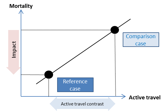
To calculate this impact, HEAT uses well-established relationships from epidemiological research between an exposure (amount of walking or cycling) and a health outcome (in HEAT: mortality from any cause: all-cause mortality). These effects are quantified as relative risks, comparing the risk (such as the risk of dying) among people who are exposed (walk or cycle regularly) to the risk among people who are not exposed (who do not walk or cycle or walk or cycle less).

The relative risk (taken from the literature) is scaled to the local levels of walking or cycling. Because relative risk estimates refer to long-term exposure, the local data provided by the user in HEAT assessment must also represent estimates of long-term walking or cycling behaviour.

The number of expected deaths in the population walking and/or cycling is calculated using the same method as above but now multiplied by the relative risk (scaled to reflect the assessed level of walking or cycling).

In a single-case assessment in HEAT, the user only specifies walking or cycling for the reference case, which is then compared to an implicit comparison case of no walking or no cycling.

In a two-case assessment, the user specifies walking and/or cycling levels for both cases.

The impact, the number of prevented premature deaths, at the population level is the difference between the calculation in the reference case and the comparison case, again reflecting population size and assessment time (see figure below.)

Figure 2 Visualization of active travel and impacts in “single case” comparative risk assessment

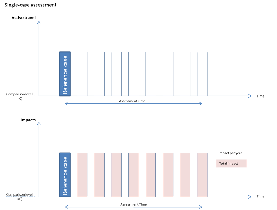
In single-case assessment, the tool assumes a steady-state situation: the assessed level of active travel is assumed to having been prevalent for several years, and subjects experience the full health effects from long-term active travel.

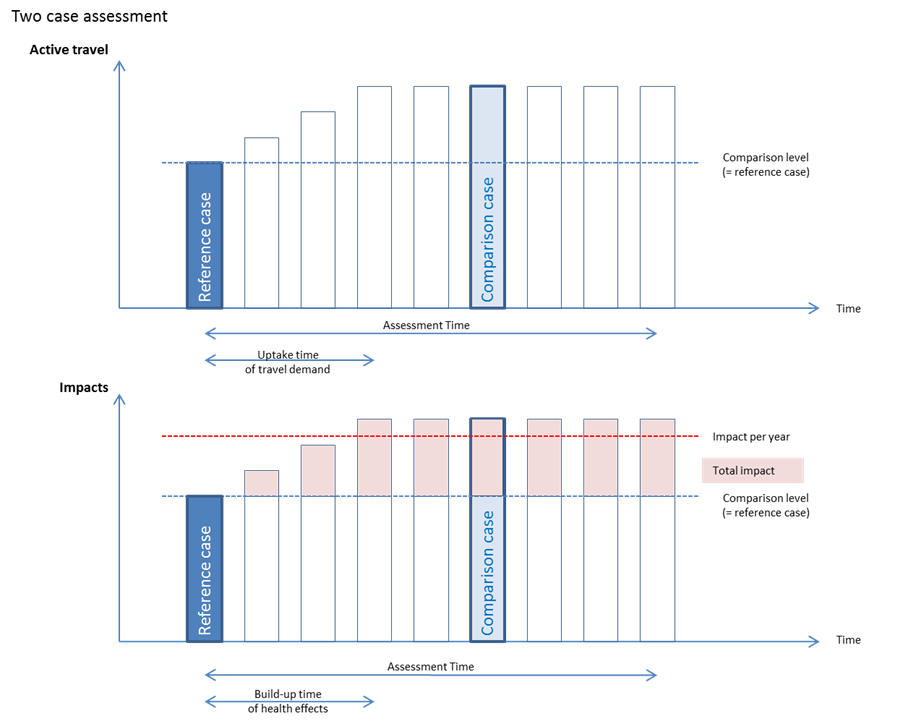
In two-case assessment, the calculations consider an uptake time until full levels of active travel are achieved (user specified) and a build-up time of five years until the health effects manifest in full (see figure below).

Figure 2 Visualization of active travel and impacts in “two case” comparative risk assessment

For detailed formulas of calculations, see here.

For more details on data needed for a HEAT assessment, see here.

For more details on assumptions that apply to HEAT assessments, see here.

Back to homepage         Back to how HEAT works

What can the tool do and what data do I need?

There are two main types of assessment in HEAT:

·       Single case assessment

o    In a "single case" assessment, only data on the so called "reference case" is provided. This is then compared to a hypothetical “comparison case” of "no walking or cycling".

o    This option is for example used when assessing the status quo, such as valuing current levels of walking and cycling in a city or country.

·       Two case assessment

o    In this case, you have to provide input data for both cases, the so called "reference case" and the "comparison case." This option is used when assessing the impact of an actual intervention or hypothetical scenarios. Typical examples are "before and after" an intervention, or comparisons of alternative "scenarios A and B" or “with measures” vs. “without measures”. 

The tool will also ask to specify:

·       if you wish to assess walking, cycling, or both;

·       geographic and time scale of the assessment;

·       type of assessment (single or two-case assessment); and

·       which impacts you wish to assess
(i.e. physical activity only, or also air pollution exposure of active travel users and/or crash risks and/or an assessment of the carbon effects of replaced motorized trips).

Before you begin, check that you have the following data available:

·       An estimate of the average amount of walking or cycling in the study population per person per day, which can come from surveys, counts or scenario assumptions. This can be entered in a number of ways, but always as an average per person and day:

o    duration (e.g. 30 minutes walked on average per day);

o    distance (e.g. 8 km cycled on average per day);

o    trips (e.g. 2 bike trips per day);

o    frequency (e.g. proportion that cycles on average 1-3 times per week)

o    mode share (e.g. on average 24% of the total traffic volume measured as distance are done by walking; here also the total traffic volume has to be entered)

o    for walking also as steps (average number of steps taken per person, e.g. 9,000 steps per day)

HEAT requires the entered data to represent long-term averages (e.g. annual averages) but allows an adjustment of the entered walking or cycling data, if necessary.

·       An estimate of the size of the assessed population. This can be either pedestrians or cyclists only, or the general population, possibly including people who do not walk or bike.  It is important that the population size refers to the same “population type” the average amounts of walking or cycling provided by the user are based on. The population size also needs to reflect the age range assessed (e.g. excluding children and young people below 20, which are not considered in HEAT assessments (see here.)

These numbers ideally come from population surveys or could be estimates, for example from scenario analyses. If route user surveys or roadside counts are used, it is important to consider that they might be affected by seasonality, weekday versus weekend behaviour, spatial variation or by other factors. These data sources also typically capture pedestrians and cyclists only, and not the general population, which must be specified when providing the amounts of walking or cycling, and considered in the population size.

·       For carbon assessments, you can also enter data on the volume of motorized modes (driving and public transport, or by more refined categories, including car (driver/passenger), motorcycle, local bus, lightrail, train). If you have no data, default values will be provided (see also below).

After you have specified your assessment type and entered your volume data, HEAT will ask some information to adjust your data for the selected impact calculations. Here some assumptions might need to be made on which no data are available, e.g. on the supposed impact of an intervention on newly induced levels of walking or cycling. You will be provided with input on such assumptions. For more information see here.

In addition, you can provide details of the cost of promoting cycling or walking, if you wish the HEAT to calculate a benefit-cost ratio. Please make sure that the costs include all relevant investments. For example, to assess the benefit-cost ratio of a promotion campaign for cycling, also think about costs for the bicycle infrastructure used by the target audience, which may be borne by the local administration.

Wherever possible HEAT provides default values (and their sources). You can use these or provide your own values if you think they more accurately reflect your situation. The most important variables are:

·       mortality rate (you can use national averages as default, or enter your local crude mortality rate);

·       value of a statistical life or social costs of carbon (you can use a European average value, or enter your local value, for more information see here

·       time period over which you wish average benefits to be calculated (which is often standardized for averaging economic assessments within a country, and where possible you should select the time period used locally);

·       a discount rate, if so wished (you can use the default value supplied or enter your own rate) (for more information see here)

A complete list of the default values for the different modules is provided here.

Back to homepage         Back to how HEAT works            Start the tool

Data sources for active travel

Data on walking or cycling come in different formats, and can be of varying quality. A few considerations will help you to make best use of your data, and avoid mistakes.

Use of short-term counts and surveys

The main concern with short-term counts is that they do not accurately capture variations in walking or cycling over time (i.e. time of the day, day of the week, season, as well as weather). If you count on a sunny day, you may see larger numbers than on a rainy day. Since HEAT assumes that the entered data reflect long-term average levels of walking or cycling, data from short-term counts will distort the results.

This issue will mainly affect single facility evaluations (e.g. a cycle path, or a pedestrian bridge) where counts are conducted on the facility itself, or community-wide evaluations that are based on surveys conducted only during a certain time of the year.

Not affected by this issue are assessments based on large surveys, which are conducted on a rolling basis (e.g. national household surveys), or automated continuous counts.

Short term counts may also be adjusted for temporal variation, to better reflect long term levels of walking or cycling. An example for how this can be done is provided by the US National Bicycle and Pedestrian Documentation Project http://bikepeddocumentation.org/

Use of data from few locations

Spatial variation in walking or cycling may affect evaluations that are based on counts at a single or few locations. The choice of location may strongly influence the count numbers, which may not be representative of the wider level of walking or cycling. Results need to be interpreted carefully, and should in general not be extrapolated beyond the locations where actual data were collected. Not affected by this issue are evaluations based on surveys that sample subjects randomly from a defined area (e.g. large household surveys), and to a lesser extent count-based evaluations on linear facilities, such as trails.

Use of trip or count data

In HEAT, trip or count data needs to be combined with an estimate for average trip length, to calculate the volume of walking or cycling. An example is counts conducted on a bridge, where it remains unknown how far people walk beyond the bridge. Average trip distance estimates may be derived from user surveys on a specific facility, or from travel surveys.

Use of pedometer data

If assessments are based on pedometer data, it should be ensured that the number of steps used is predominantly composed of intentional brisk walking. Some pedometers have a function that excludes steps that are not deliberate walking. Another approach could be to include only intentional walking steps at a rate of about 100 steps per minute or to make an assumption of the proportion of total steps falling into this category.

Back to homepage         Back to data needs

Conversion of input units for travel volume data

While HEAT requires volume data to be inserted as “per person and day”, it allows the user to insert their data on travel modes in various units or formats. The tool then converts these to standard units, such as minutes and kilometres per day. Default values are used to inform these conversions as necessary (e.g. average trip distance).

The following input formats (per person per day) are supported:

·       duration: average time (minutes or hours) walked or cycled per person, such as 30 minutes walked on average per day;

·       distance: average distance walked or cycled per person, such as 10 km cycled on average per day;

·       trips: average per person or total observed across a population, such as 250 bicycle trips per year;

·       steps: average number of steps taken per person, such as 9000 steps per day;

·       mode share (in trips, duration or distance): mode share is a percentage of total travel (all modes): for example, 20% of all trips are walking;

·       frequency, referring to such questions as “How often do you use your bike?” or “How often do you walk?” (such as 20% if users cycle 1–3 days per week); and

·       percentage change: for example, compared with scenario A, in scenario B 20% of the population cycles x minutes more.

The following conversions apply:

·       To convert volume data between duration and distance, average speeds by transport mode are assumed (see here)

·       To convert steps into distance, the number of steps is multiplied by an average default step length (see here).

·       To convert number of trips into distance, average trips distances by transport mode are used (see here).

·       To convert mode share, the percent share is multiplied by the total volume (trips, distance or duration) and then the conversions as described above are applied, as necessary.

·       The following frequency categories are available: daily or almost daily, 1–3 days per week, 1–3 days per month, less than once per month and never. To convert frequency categories into distances, first the number of days walked or cycled per year is derived, using the category midpoints.

Thus, “daily or almost daily” is assigned 5.5 days per week (midpoint between 7 and 4 days in a week) and multiplied by 52; “1–3 days per week” is assigned 2 days per week; “1–3 days per month” is assigned 2 days per month and multiplied by 12; “less than once per month” is 6 days per year; and “never” is assigned zero. The days per year are then divided by 365 and multiplied by an average daily distance by mode , which is estimated by multiplying a number of trips per person per day in all modes (three) by the average trip distance by mode.

·       The input option “percent change” is available for two case assessments and allows specifying the comparison case in terms of relative change from the reference case.

Back to homepage         Back to data needs

Data adjustments for the HEAT calculations

Input data on active modes of transport provided by the user may not be adequate or sufficient for all calculations of impact. HEAT therefore offers several options to adjust the data or provide additional information to inform the calculation, depending on the characteristics of the assessment. If the user does not provide such information, default settings apply.

Data adjustment options in HEAT may include the following (depending on the type of assessment):

·       proportion excluded

·       temporal and spatial adjustment

·       uptake time for active travel demand

·       proportion of new trips

·       proportion of reassigned trips

·       proportion of shifted trips

·       proportion in traffic

·       proportion for transport

·       traffic conditions

·       change in crash risk

·       substitution of physical activity.

General adjustments of active travel data

Proportion excluded due to unrelated factors (“two case assessments” only)

When the impact of an intervention is assessed, not all the cycling or walking observed may be directly attributable to the intervention. For example, cycling may have become more fashionable over time, or gasoline or public transport prices may have changed and affected active transport behaviour. Walking or cycling arising from such external effects should not be included in the assessment of the infrastructure or project.

The precise effects of an intervention and unrelated factors can rarely be disentangled. Estimate the proportion you would exclude from the assessment (such as –30%) to the best of your knowledge. For more guidance on this, see also here.

The default setting is 0%.

Temporal and spatial adjustment

HEAT requires long-term average input on active travel (such as annual means). Active travel is highly affected by such factors as season, weather and time of day. Short-term counting, for example, is typically carried out in summer or fall and often during rush hour. If active travel data is from a short-term survey or count, it likely under- or overestimates the long-term average. This can be adjusted here (such as + 20% or – 30%). Data from continuous counters can be helpful in assessing the potential need for adjusting for time.

Similarly, the location where count data or intercept surveys are collected may not represent average volumes for the complete facility of interest (such as a bike path, trail, or network). This slider can be used to apply a spatial adjustment (such as + 20% or – 30%). Data from multiple locations are usually needed to inform spatial adjustment, but crude guesses may be adequate in some cases. Accurate spatial adjustment would require a spatial modelling approach.

The default setting is 0%.

Uptake time for active travel demand (“two case assessments” only)

Here users can specify a take-up time (in years) until the maximum volume of active travel is reached. This allows adjusting for the estimated time to reach the full level of walking or cycling entered, such as after an intervention has been implemented. For example, if a new footpath is built, and an estimated 5 years will elapse for usage to reach a steady state, this figure should be changed to 5. For steady-state situations, with no build-up time considered, this should be set to zero.

The default setting is 1 year.

Investment costs (“two case assessments” only)

This input field allows the user to provide an estimated cost for the investment that led to the assessed active travel. HEAT will compare this to the monetized value of the effects and calculate a benefit–cost ratio.

Information to characterize the contrast between reference and comparison case

HEAT assessments are based on a comparison between the reference and the comparison case (more on this here). In a two-case comparison, the user provides travel data for both cases. In single-case assessment, users do not provide input data for the comparison case, leaving a greater information gap for the HEAT assessment. To improve the calculations for certain types of assessment (use cases), HEAT allows the comparison to be informed using some additional questions. HEAT automatically only presents the questions needed for assessment.

A first set of questions asks “if, where and how the trips in the reference case would occur in the comparison case”. The three questions specifically request the proportion of new trips, reassigned trips and shifted trips.

Proportion of new trips (“two case assessments, carbon” only)

New trips are trips that did not take place in the comparison case: they were neither shifted from another mode nor reassigned from another route. This information is captured through other entry options for physical activity, air pollution and road crash assessment. For carbon emission assessment for which no motorized input data are available, this additional information is needed to adjust the cold-start emissions, which are calculated based on the number of trips by active mode per year (see operational emissions).

The default setting is 0%.

Proportion of reassigned trips (“two case assessments, sub-city level” only)

Reassigned trips are trips that merely follow a different route to now take place using new infrastructure (such as a new footpath or a cycling network). These reassigned trips will not be considered in the assessment because they do not reflect a net increase in active travel. The percentage of reassigned trips has to be estimated, unless a specific survey has been carried out before the new infrastructure has been put into place (asking for example: “Prior to this facility being built, did you use a different route for this trip?" or "Prior to this infrastructure being built, did you also use your bike for this particular kind of trip (e.g. to work, or for recreation)?”). It is likely that the percentage is higher on very attractive new facilities (e.g. a nice bike path) or which play a key role in the network (e.g. a bridge), and lower on less attractive facilities (e.g. a stretch of sidewalk).

This adjustment will only be applied to sub-city-level assessments, since trips cannot be reassigned for countrywide or citywide assessment.

The default setting is 0%.

Proportion of trips shifted from another mode (“single case assessments, carbon” only)

Shifted trips are active mode trips that replace a trip by another mode in the comparison case. Users are first asked to provide the total proportion shifted (such as 80%).

The default setting is 0%.

Thereafter users can specify the other mode of active travel from which was shifted. The sum of the modal shift percentages cannot add up to more than 100%  (see more information on carbon emissions assessment).

These sliders are set to default values, which will apply if no adjustments are made.

Other adjustments

Motorized traffic influences both carbon emissions and exposure to air pollution. Three questions capture the relevant information:

Proportion of active travel done “in traffic” (“air pollution assessments” only)

This question asks what proportion of active travel (in the reference case) takes place in traffic (versus away from major roads, in parks etc.) and adjusts accordingly the air pollution levels to which the cyclists or pedestrians being assessed are exposed (see more information here.

The default setting is 50%.

Proportion of travel done “for transport” (“air pollution and carbon assessments” only)

This information is used to correctly assign air pollution concentrations in the comparison case. Trips for transport are assumed to replace modes of transport (time in traffic environments with higher air pollution concentrations), whereas recreational trips replace time at home (at background air pollution concentrations). Transport-related means to get to and from places, to pursue a specific purpose at the destination (such as work, shop, visit friends or play tennis). Recreation means that the main purpose of the trip is exercise or recreation. Please specify the proportion of the travel entered that is for transport purposes (versus for recreation).

For more information on air pollution assessments, see here.

For carbon assessment, only active travel for the purpose of transport is considered, presuming that it replaces other modes of transport. Recreational trips are presumed not to replace other modes of transport.

For more information on carbon emission assessments, see here.

The default setting is 50%.

Traffic conditions (“carbon assessments” only)

For carbon emission assessment, users are also asked to specify the local traffic conditions, referring to the times when people walk or cycle. Traffic conditions affect carbon emission rates. Users can select between European average (urban and rural), free flow (little or no congestion, 45 km/h mean traffic speed), some peak-time congestion (morning commute, school run, afternoon commute, 35 km/h mean traffic speed) or heavy congestion on most days (20 km/h mean traffic speed).

The default setting is European urban average.

Change in crash risk (“two case assessments, crashes” only)

The road crash risk for active modes of transport depends, among many other factors, on the volume of walking or cycling (also called safety in numbers). To consider a change in road crash risk between the two comparison cases, specify it here as a percentage change relative to the reference case. Leaving this blank will apply the same road crash risk to both cases. The changes in road crash risk may result from an increase in active modes, improved infrastructure or any other reason.

The default setting is 0%.

Substitution effect (“two case assessments, physical activity” only)

In some cases, some of the observed cycling or walking may substitute for other physical activity, such as sport previously done in leisure time. This proportion does not contribute to a net gain in physical activity and should be excluded from the assessment.

The default setting is 0%.

Back to homepage         Back to how HEAT works            Back to data needs

Proportion of cycling or walking excluded due to unrelated factors

When the impact of an intervention is assessed (two case assessments only), not all the cycling or walking observed may be directly attributable to the intervention. For example, cycling may have become more fashionable over time, or gasoline or public transport prices may have changed and affected active transport behaviour. Walking or cycling arising from such external effects should not be included in the assessment of the infrastructure or project. This is sometimes also referred to as the change that would happen anyway under the “business-as-usual” scenario.

Figure 1 Effects of measure (intervention) versus other unrelated effects (from Evaluation matters.)

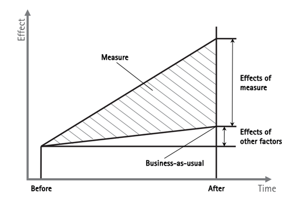
This unrelated proportion can be excluded using this slider (default setting 0%).

Suggested values:

Close to 0 (0-30%):
Assessments of comprehensive long-term measures, system-wide (i.e. whole communities), unaffected by major other factors that could have influenced cycling or walking (e.g. without major increases of fuel or public transport prices).

Mid-range (30-80%):
This applies to assessments where there is belief that other factors than the evaluated interventions have contributed towards the observed changes in cycling or walking. Examples are increases in cycling or walking which were accompanied by steep increases in fuel prices, or when assessing a specific measure that was implemented during the same time as other measures affecting walking or cycling.

High range (>80%):
Excluding more than 80% of observed walking or cycling due to unrelated factors may probably only be applied for unusual circumstances, when you have strong evidence that a change in active travel you observe within your assessment project is attributable to a more impactful outside factor. For example, if you assess the impacts of a particular piece of infrastructure, but at the same time speed limits have been reduced area-wide, which presumably has a stronger effect on active travel.

Back to homepage         Back to how HEAT works            Back to data adjustments

How do the HEAT assessments work?

HEAT allows to calculate the mortality benefits of regular physical activity from cycling or walking only (like the previous versions of HEAT), or to take into account the effects of air pollution and crashes or to estimate the carbon emission effects from replacing motorized trips by walking or cycling.

More information on each of these modules can be found in the subsequent pages.

Back to homepage         Back to start using the tool

Mortality impact calculation for physical activity and air pollution pathways

The HEAT impact calculations for physical activity and air pollution apply a population attributable fraction (PAF) formula. This formula is used to relate the mortality rate for the general population (MR_pop) to the two groups compared in comparative risk assessment:  the exposed group (reference group) (e) and unexposed group (comparison group) (u). In HEAT, exposure refers to the assessed amount of cycling or walking.

The MRpop is the weighted average of the mortality rate in the exposed (MRe) and unexposed (MRu). MRpop depends of the contrast in mortality risk between the two groups, as well as the size of the two groups.

MRpop = MRu x Pu + MRe x Pe

Epidemiological studies estimate the contrast in mortality risk and express it as a relative risk (RR): for example, RRcycling = 0.9 for x minutes of cycling per day compared with 0 minutes of cycling per day).

RR = MRe/MRu

The size of the exposed and unexposed groups is typically expressed as the proportion of exposed subjects (Pe). In the HEAT context, this quantifies the size of the assessed population cycling or walking relative to the size of the total population on which the MRpop is based (all inhabitants of a country 20–64 or 20–74 years old, respectively). In most use cases, the proportion of people exposed is quite small, such as in city-level or sub-city-level assessment (in which the population assessed is much smaller than the country’s population), and in assessments in which walking or cycling levels are not very high (with little influence on the overall mortality risk). By default, the tool therefore assumes the proportion of exposed people to be close to zero (0.001), which means that the influence of the assessed walking or cycling on the country-level mortality rate (MRpop) is negligible. Users may change this for use cases in which this does not apply, such as country-level assessments in which walking and cycling levels are very high. In these cases, mode share or an equivalent figure can be used as an approximation of the proportion exposed.

The mathematical formulas used by HEAT were derived based on these considerations. To calculate effects in terms of premature deaths (avoided), MRu and MRe are estimated based on MRpop, RR, (and Pe~=0).

MRpop = MRu x Pu + MRe x Pe

RR = MRe/MRu

Pu = 1-Pe

MRu = MRpop / [1 – (Pe*(1 – RR))] ~= MRpop

MRe = MRpop x RR / [1 – (Pe x (1 – RR))] ~= MRpop x RR

MRu and MRe are then multiplied by the assessed population to derive the number of deaths in the exposed group (the population assessed in HEAT) and unexposed group (the hypothetical counterfactual of the same population not being exposed: not cycling or walking). The difference between the two groups reflects the number of deaths attributed to the exposure or the impact of the exposure. If the impact is smaller among exposed people, the exposure prevents deaths, such as physical activity.

Du = MRu x pop

De = MRe*pop

D_attributed = De – Du

In a two-case comparison, the same assessment is calculated twice for different levels of exposure. The deaths attributed then reflect the difference between the two assessments.

More information on how the different HEAT modules calculate impact assessments can be found here.

Back to homepage         Back to how HEAT works            Back to health impact assessment intro

Basic function of the HEAT for walking and cycling

HEAT applies 5 key steps as shown in the figure below.  

Figure: Functioning of the HEAT for walking and cycling in 5 steps

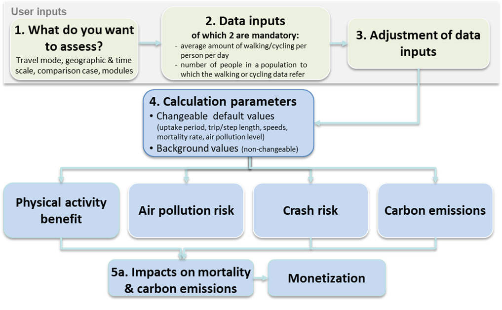
For a detailed description of the steps, please refer to the pages on how HEAT works, or to chapter 3 and 4 of the HEAT methods and user guide booklet.

Back to homepage         Back to how HEAT works

Physical activity assessment in HEAT

To derive an estimate of the health benefits from physical activity from regular walking or cycling, the tool uses estimates of the relative risk of death from any cause among regular cyclists or walkers compared with people who do not cycle or walk regularly.

The tool is based on a relative risk from a meta-analysis of published studies. For more details on the relative risks used in HEAT for cycling and walking, see here.

The tool uses these relative risks and applies them to the amount of walking or cycling entered by the user, assuming a linear relationship between walking or cycling and mortality. To illustrate this, the relative risk from the meta-analysis used for the updated version of HEAT for cycling is 0.90 for regular commuter cycling for 100 minutes per week for 52 weeks of the year (equivalent to 87 hours of cycling per year). Thus, in any given year, a population of regular cyclists receives a protective benefit of 10% (1.00 minus 0.90): that is, overall they are 10% less likely to die from all causes combined than a population of non-cyclists. If the user enters a cycling volume equivalent to 29 hours per year (one third as much), the protective benefit of this amount of cycling will be about 3%. If the user enters 174 hours (twice the time cycled in the reference population), the resulting protective benefit is 20%. This is twice the protective benefit of the reference population.

The same approach is taken for walking, in which the risk reduction is 0.89 for regular walking of 168 minutes per week for 52 weeks of the year (equivalent to 146 hours of walking per year). HEAT then uses population-level mortality data to estimate the number of adults normally expected to die in any given year in the target population. Then it calculates the reduction in expected deaths among the people in this population who cycle or walk at the level specified by the user, using the adjusted relative risk.

Unless a steady-state situation is being assessed, it is important to recognize that there will be a time lag between increases in physical activity and measurable benefits to health. Based on expert consensus, it was agreed that five years was a reasonable assumption to use for such additional physical activity to reach full effect, with an increment of 20% in benefits each year.

Scope and limitations

Although literature suggests that the dose–response relationship between physical activity and mortality is most likely non-linear (2,3), the meta-analysis carried out for HEAT (1) also showed that differences between various dose–response curves were modest (see also here). For HEAT, a linear relationship was chosen to avoid additional data requirements on baseline activity levels (which would be needed using a non-linear dose–response function) and because a linear approximation is often adequate within the foreseen range of activity for HEAT

To avoid inflated values at the upper end of the range, the risk reduction available from HEAT is capped. Inspection of the data points of the new meta-analyses suggested that, after about 45% risk reduction for cycling and 30% for walking, the risk reduction starts to slow (and most of the evidence relates to exposure below these levels). A large cohort study found through purposive review (4) also confirmed these limits. On this basis, the advisory group recommended using these caps in the updated HEAT. Thus, HEAT will apply a maximum 45% risk reduction (corresponding to 447 minutes per week) in the risk of mortality for cycling and a maximum 30% risk reduction (corresponding to 460 minutes per week) for walking.

Table: Caps for the benefits from physical activity in HEAT

CI: confidence interval.

Formula

The basic functioning of the physical activity module of HEAT is shown in the figure below:

(1-RR)×((Local volume of walking/cycling)/(Reference volume walking/cycling))             Where:

RR = relative risk of death in underlying studies (walking: 0.89; cycling: 0.90)

Reference volume of cycling per person calculated based on 100 minutes per week for 52 weeks per year at an estimated speed of 14 km/hour.

Reference volume of walking based on 168 minutes per week at 5.3 km/hour

The relative risk is then used to calculate number of deaths prevented based on mortality rate, applying a population-attributable fraction formula. For details, see here.

Back to homepage         Back to how HEAT works            Back to how HEAT assessments work

Sources:

1.        Kelly P et al. Systematic review and meta-analysis of reduction in all-cause mortality from walking and cycling and shape of dose response relationship. 2014, International Journal of Behavioral Nutrition and Physical Activity (11):132 (https://doi.org/10.1186/s12966-014-0132-x, accessed 31 August 2017).

2.        Woodcock J et al. Non-vigorous physical activity and all-cause mortality: systematic review and meta-analysis of cohort studies. Int J Epidemiol. 2011;40:121–38

3.        Wen CP et al. Minimum amount of physical activity for reduced mortality and extended life expectancy: a prospective cohort study. Lancet. 2011;378:1244–53.

4.        Manson J et al. Walking compared with vigorous exercise for the prevention of cardiovascular events in women. 2002, N Engl J Med, 347(10): 716-725.

Relative risk estimate used in the HEAT for physical activity assessments

The strongest evidence at the time of the first project on the mortality effects of cycling was the relative risk data from two combined Copenhagen cohort studies (1,2,3). This study included about 7000 20- to 60-year-old participants followed up for an average of 14.5 years. It found a relative risk of all-cause mortality among regular commuter cyclists of 0.72 (95% CI 0.57–0.91) compared with non-cycling commuters for 180 minutes of commuter cycling per week.

In 2013, a new systematic review on the reduced relative risk of all-cause mortality from regular cycling or walking was carried out (4).

To be included in this review, a study was required:

·       to be a prospective cohort study;

·       to report the level of regular walking or cycling (such as duration, distance or MET equivalent);

·       report all-cause mortality rates or risk reductions as outcome; and

·       report results independent of (that is, adjusted for) other physical activity.

A total of 8901 titles were identified, and 431 full texts were screened. Seven cycling studies (carried out in China, Denmark, Germany and the United Kingdom) and 14 walking studies (from China, Denmark, Germany, Japan, United Kingdom and the United States) met the inclusion criteria. A meta-analysis was carried out, combining the results of these studies. Since the available studies used a range of types of exposure, conducting the meta-analysis required estimated for each study the reduced risk at a common exposure level. For this purpose, the various types of cycling and walking exposure used in the studies were converted into MET-hours per week (assuming a linear dose–response relationship and an average intensity of 6.8 METs for cycling and 4.0 METs for walking, if not otherwise stated). The common exposure level was set at 11.25 MET-hours per week. This value was derived from the global physical activity recommendations as corresponding to the recommended level of at least 150 minutes of moderate-intensity physical activity per week (5) using 4.5 METs as an average for moderate-intensity physical activity. Using 6.8 METs as an average intensity for cycling, this exposure represents about 100 minutes of cycling per week and 170 minutes of walking per week, using an average intensity of 4.0 METs.

The international advisory group recommended that, for HEAT, a linear dose–response curve based on a relative risk of 0.90 for cycling and 0.89 for walking should be used, applying a constant absolute risk reduction (6). The sensitivity of the results to various possible shapes of dose–response relationships was tested. The differences between the various curves were modest, and the difference in the final risk estimate was no more than 6%.

Combining physical activity and air pollution exposure

The published relative risks for mortality and physically activity from walking and cycling used by HEAT are taken from studies in settings in which participants were exposed to (different levels of) air pollution. As such, the relative risks for physical activity include a small population-average degree of influence of air pollution while walking or cycling. When HEAT users select solely assessing the effects of physical activity, this is not specifically adjusted for, implicitly assuming that air pollution levels are comparable between the assessed setting and the settings in which the studies were conducted.

However, if the user selects both the physical activity and the air pollution assessment, then HEAT adjusts the relative risk for physical activity benefits from walking and cycling to exclude the effects of air pollution, using relative risk estimates adjusted to what they would be if the physical activity studies had been conducted in non-polluted environments. The effects of the additional air pollution exposure from walking or cycling are calculated separately (and shown in the detailed HEAT results).

To derive the adjusted relative risks, the exposure to air pollution (PM2.5) in each of the cycling and walking study settings was estimated using international databases and assuming a 50% higher historical exposure to consider the general improvement of air pollution between the time the underlying studies were conducted (between 1964 and the early 2000s) and the year 2011 for which air pollution exposure was available (7). The effect of this exposure while walking or cycling on the original relative risks from the physical activity studies (4) was calculated, using a published exposure response function between PM 2.5 and all-cause mortality (8), default inhalation rates and the published durations of exposure (4).

Overview of the relative risks used in physical activity assessments

Cycling

·       Unadjusted: RR = 0.903 (0.866-0.943)

·       Adjusted for air pollution (new): RR = 0.899 (0.861-0.939)

Walking

·       Unadjusted: RR = 0.886 (0.806-0.973)

·       Adjusted for air pollution (new): RR = 0.883 (0.803-0.970).

Note that the vice versa argument could be made for the influence of active travel on the published relative risks of air pollution from studies in which subjects engaged in walking or cycling. It is fair to assume that this influence would be negligible because of the small contribution of the additional inhaled dose of air pollution while walking or cycling to the total exposure of the entire study population.

Back to homepage         Back to how HEAT works            Back to how HEAT assessments work

Sources:

1.        Andersen LB et al. All-cause mortality associated with physical activity during leisure time, work, sports and cycling to work. Arch Intern Med. 2000;160:1621–8.

2.        Rutter H et al. Economic impact of reduced mortality due to increased cycling. Am J Prev Med. 2013;44:89–92.

3.        Kahlmeier S et al. Health economic assessment tools (HEAT) for cycling and walking. Methodology and user guide. Copenhagen: WHO Regional Office for Europe; 2011 (http://www.heatwalkingcycling.org/ index.php?pg=archive, accessed 26 March 2014).

4.        Kelly P et al. Systematic review and meta-analysis of reduction in all-cause mortality from walking and cycling and shape of dose response relationship. 2014, International Journal of Behavioral Nutrition and Physical Activity (11):132 (https://doi.org/10.1186/s12966-014-0132-x, accessed 31 August 2017).

5.        Global recommendations on physical activity for health. Geneva: World Health Organization; 2010 (http://www.who.int/dietphysicalactivity/factsheet_recommendations/en/index.html, accessed 26 March 2014).

6.        Development of guidance and a practical tool for economic assessment of health effects from walking. Consensus workshop, 1–2 July 2010, Oxford, United Kingdom. Background document: summary of literature reviews and issues for discussion. Copenhagen: WHO Regional Office for Europe; 2010.

7.        Development of the Health economic assessment tools (HEAT) for walking and cycling: Consensus workshop. Meeting background document. Bonn, Germany, 11-12 December 2014. Copenhagen: WHO Regional Office for Europe; 2014.

8.        Hoek G et al. Long-term air pollution exposure and cardio- respiratory mortality: a review. Environ Health. 2013 May 28;12(1):43.

Air pollution assessment in HEAT

A method used for quantitative risk assessment of air pollution and modes of transport (1,2) was agreed to serve as basis for assessing the air pollution effects on cyclists and pedestrians in HEAT (3,4, 5). Based on the selected country and/or city, HEAT will propose a PM2.5 level retrieved from the WHO Global Urban Ambient Air Pollution Database (city values) (6) or the Global Health Observatory data repository (country values) (7); users can review this value. If no value is available from the databases or the user prefers to enter a local value, a PM2.5 value can be entered (or a PM2.5 value can be derived using an internationally accepted conversion factor of 0.6 (8) to transform more widely available PM10 measurements into estimates of PM2.5 (4), where necessary).

The equivalent change of air pollution intake resulting from cycling or walking compared with a reference scenario is calculated using a ventilation rate (1.37 m3/hour for walking and 2.55 m3/hour for cycling) (3,4), duration of exposure and PM2.5 concentrations in the mode of transport. The calculated intake is added to the intake during the rest of the day.

HEAT considers two aspects when calculating the difference in air pollution exposure resulting from a specific level of cycling or walking:

1.      the location of the cycling or walking to derive the appropriate level of air pollution exposure:

o    mainly on or near a road with motorized traffic (and therefore at an air pollution concentration that is considered equal to the background concentration multiplied by an agreed conversion factor for cycling or walking (see below));

o    (b) mainly in a park or away from roads with motorized traffic (and therefore at a concentration of air pollution that could be considered equal to the background concentration); an (see below).

2.      the main purpose of the cycling and walking to derive the appropriate reference case:

o    mainly for leisure where the comparison scenario HEAT is using is “staying at home” (with a concentration of air pollution that is considered to be equal to background concentration and a ventilation rate of 0.61 m³/hour);

o    (b) mainly for commuting where the comparison scenario for HEAT is “using a car” (with a concentration of air pollution equal to the background concentration multiplied by an agreed conversion factor (see below) and a ventilation rate of 0.61 m³/hour (3,4)).

Mode-specific PM2.5 concentrations are derived from the background concentrations using conversion factors. The applied factors of 2.0 for cycling, 1.6 for walking and 2.5 for using a car^* (versus background) were derived for HEAT from a purposive review of studies that estimated PM2.5 concentrations while cycling or walking compared with concentrations in other modes of transport (9).

The international advisory group for use in HEAT agreed to use a meta-analysis including 14 international cohort studies, which summarized the relative risk between all-cause mortality and each increment of 10 µg/m3 of PM2.5 as 1.07 (1.04–1.09) (4). It is important to recognize that there will be a time lag between exposure to air pollution and negative health effects. Based on expert consensus, a time lag of 5 years – similar to that used for health effects from physical activity (see also here) – will be used for air pollution effects to build up on mortality as a reasonable and most likely conservative assumption, with an increment of 20% in benefits each year.

Scope and limitations

The use of non-linear integrated dose–response functions has been suggested to reflect indications that the relationship between air pollutants and health risk seem to become flat at higher pollution levels (4). However, HEAT is being proposed predominantly for applications in the European Region, where the extreme exposure sometimes found in other parts of the world is rare. The experts therefore adopted a linear dose–response function as being appropriate within the HEAT framework (5).

To avoid inflated values at the upper end of the range, the risk increase from exposure to particulate matter within HEAT is capped. A previously used cap of 50 µg/m3 (10) was agreed to use for HEAT, which is also in accordance with the evidence on the air pollution exposure in the locations in which the studies took place that HEAT is based on (see here). Although HEAT still applies to locations with somewhat higher levels of air pollution, in this case no further health effects will be applied beyond 50 µg/m3. No lower cap is used for HEAT, as recent evidence shows that health effects also occur at very low concentrations of air pollution (11).  

Finally, HEAT only includes air pollution effects among cyclists and pedestrians and does not consider the (often substantial (1)) effects of reducing air pollution for the whole population by replacing motorized transport by cycling and walking.

^* The literature review (9) focused on studies contrasting active vs. passive travel modes; the car vs. background ratio used in HEAT is stemming from the studies included in this review and should be seen as an approximation.

Back to homepage         Back to how HEAT works            Back to how HEAT assessments work

Sources:

1.        de Hartog JJ et al. Do the health benefits of cycling outweigh the risks? Environ Health Perspect. 2010;118:1109–16.

2.        Rojas-Rueda D et al. The health risks and benefits of cycling in urban environments compared with car use: health impact assessment study. BMJ. 2011;343:d4521.

3.        Rojas-Rueda D, Nieuwenhuijsen M. Adjustment of risk estimates of physical activity and mortality by the impact of air pollution (particulate matter of less than 2.5 µm). Barcelona: Centre for Research in Environmental Epidemiology (CREAL); 2014.

4.        WHO expert meeting: methods and tools for assessing the health risks of air pollution at local, national and international level. Meeting report, Bonn, Germany, 12–13 May 2014. Copenhagen: WHO Regional Office for Europe; 2014 (http://www.euro.who.int/en/health-topics/environment-and-health/air-quality/publications/2014/who-expert-meeting-methods-and-tools-for-assessing-the-health-risks-of-air-pollution-at-local,-national-and-international-level, accessed 26 June 2015).

5.        Development of the health economic assessment tools (HEAT) for walking and cycling. Consensus workshop. Bonn, Germany, 11–12 December 2014. Copenhagen: WHO Regional Office for Europe; 2015.

6.        World Health Organization. WHO Global Urban Ambient Air Pollution Database (http://www.who.int/phe/health_topics/outdoorair/databases/cities/en/), accessed 14 September 2017.

7.        World Health Organization. WHO Global Health Observatory data repository, Exposure Country Average 2014. (http://apps.who.int/gho/data/view.main.SDGPM25116v?lang=en), accessed 15 September 2017.

8.        PM2.5, an indicator for fine particles. In: Air quality guidelines. Global update 2005. Particulate matter, ozone, nitrogen dioxide and sulfur dioxide. Copenhagen: WHO Regional Office for Europe, 2006: 40–1 (http://www.who.int/phe/health_topics/outdoorair/outdoorair_aqg/en, accessed 26 June 2015).

9.        De Nazelle et al. Comparison of air pollution exposures in active vs. passive travel modes in European cities: A quantitative review. Environment International 2017 (99): 151-160 (Appendix C). (http://www.sciencedirect.com/science/article/pii/S0160412016304585?via%3Dihub, accessed 31 August 2017).

10.     Cohen A et al. Urban air pollution. In: Ezzati M, Lopez AD, Rodgers A, Murray CJL, editors. Comparative quantification of health risks: global and regional burden of disease attribution to selected major risk factors. Volume 1. Geneva: World Health Organization; 2004:1353–434. (http://www.who.int/healthinfo/global_burden_disease/cra/en, accessed 31 August 2017).

11.     Di Q et al. Air Pollution and Mortality in the Medicare Population. N Engl J Med 2017; 376:2513-2522, 2017DOI: 10.1056/NEJMoa1702747.  

Air pollution in HEAT

Air pollution is a complex mixture of different components. Particle pollution (also known as particulate matter) in the air includes a mixture of solids and liquid droplets. Some particles are emitted directly; others are formed in the atmosphere when other pollutants react. Particles come in a wide range of sizes. Those less than 10 micrometres in diameter (PM10) are so small that they can get into the lungs, potentially causing serious health problems. Even stronger health effects have been shown for particles with a diameter of less than 2.5 micrometres (PM2.5). Based on a large body of evidence, mainly from cohort studies and the relatively good availability of data on particulate matter, PM2.5 was proposed as the indicator of air pollution to estimate the related health effects for HEAT.

In the absence of local PM2.5 concentration measurements, an internationally accepted conversion factor of 0.60 was agreed (1) to use for HEAT to transform more widely available PM10 measurements into estimates of PM2.5 (more information on background values.)

Since evidence shows that PM2.5 is less directly related to emissions from road traffic than other pollutants, such as elemental carbon or black smoke, a sensitivity analysis was carried out (2) to assess the influence of the choice of pollutant on the HEAT results. Using elemental carbon, the estimates were very similar to those based on PM2.5.

For more information on air pollution see here.

Back to homepage         Back to how HEAT works            Back to air pollution assessment

Sources:

1.        PM_2.5, an indicator for fine particles. In: Air quality guidelines. Global update 2005. Particulate matter, ozone, nitrogen dioxide and sulfur dioxide. Copenhagen: WHO Regional Office for Europe, 2006: 40–1 (http://www.who.int/phe/health_topics/outdoorair/outdoorair_aqg/en, accessed 26 June 2015).

2.        Development of the health economic assessment tools (HEAT) for walking and cycling. Consensus workshop. Bonn, Germany, 11–12 December 2014. Copenhagen: WHO Regional Office for Europe; 2015.

Relative risk estimates used in the HEAT impact assessment of exposure to air pollution while walking or cycling

HEAT uses a relative risk from a meta-analysis including 14 international cohort studies from the Austria, Canada, Denmark, France, Finland, Germany, Greece, Italy, the Netherlands, Norway, Spain, Sweden, Switzerland, the United Kingdom and the United States (1). It quantifies the relative risk for mortality from all causes for each increment of 10ug/m3 of PM2.5 (particulate matter with a diameter of less than 2.5 micrometres (see also here) as 1.07 (confidence interval: 1.04-1.09). This translates into a 7% increase in risk of dying per each additional increase in long-term exposer to 10ug/m3 PM2.5. In other words, people who are exposed to PM2.5 levels that are 10ug/m3 higher, have a 7% increased risk of dying (at any point in time) than people who are exposed to 10ug/m3 less, assuming they do not differ in age, smoking status, or any other relevant characteristic.

If multiple papers on a study existed, only the most recent one was used, which had longer follow-up. The only studies included in the quantitative meta-analysis were those that directly estimated PM2.5 exposure. For all-cause mortality from PM2.5 exposure, the initial analysis (4) included 11 studies and was later updated including 3 more studies (1), which only had a minor effect on the relative risk estimate.

The authors also found little evidence for a stronger association among women than among men. People with less education and obese subjects had a larger estimated effect for mortality related to fine particulate matter, although more recent studies have weaker evidence for differences related to education (4).

Combining physical activity and air pollution exposure

The published relative risks for mortality and physically activity from walking and cycling used by HEAT are taken from studies in settings in which participants were exposed to (different levels of) air pollution. As such, the relative risks for physical activity include a small population-average degree of influence of air pollution while walking or cycling. When HEAT users select solely assessing the effects of physical activity, this is not specifically adjusted for, implicitly assuming that air pollution levels are comparable between the assessed setting and the settings in which the studies were conducted.

However, if the user selects both the physical activity and the air pollution assessment, then HEAT adjusts the relative risk for physical activity benefits from walking and cycling to exclude the effects of air pollution, using relative risk estimates adjusted to what they would be if the physical activity studies had been conducted in non-polluted environments. The effects of the additional air pollution exposure from walking or cycling are calculated separately (and shown in the detailed HEAT results).

To derive the adjusted relative risks, the exposure to air pollution (PM2.5) in each of the cycling and walking study settings was estimated using international databases and assuming a 50% higher historical exposure to consider the general improvement of air pollution between the time the underlying studies were conducted (between 1964 and the early 2000s) and the year 2011 for which air pollution exposure was available (2). The effect of this exposure while walking or cycling on the original relative risks from the physical activity studies (3) was calculated, using a published exposure response function between PM 2.5 and all-cause mortality (4), default inhalation rates and the published durations of exposure (3).

Overview of the relative risks used in physical activity assessments

Cycling

·       Unadjusted: RR = 0.903 (0.866-0.943)

·       Adjusted for air pollution (new): RR = 0.899 (0.861-0.939)

Walking

·       Unadjusted: RR = 0.886 (0.806-0.973)

·       Adjusted for air pollution (new): RR = 0.883 (0.803-0.970).

Note that the vice versa argument could be made for the influence of active travel on the published relative risks of air pollution from studies in which subjects engaged in walking or cycling. It is fair to assume that this influence would be negligible because of the small contribution of the additional inhaled dose of air pollution while walking or cycling to the total exposure of the entire study population.

Back to homepage         Back to how HEAT works            Back to air pollution assessment

Sources:

1.        PM2.5, an indicator for fine particles. In: Air quality guidelines. Global update 2005. Particulate matter, ozone, nitrogen dioxide and sulfur dioxide. Copenhagen: WHO Regional Office for Europe, 2006: 40–1 http://www.euro.who.int/__data/assets/pdf_file/0010/263629/WHO-Expert-Meeting-Methods-and-tools-for-assessing-the-health-risks-of-air-pollution-at-local,-national-and-international-level.pdf?ua=1, accessed 10 October 2017).

2.        Development of the Health economic assessment tools (HEAT) for walking and cycling: Consensus workshop. Meeting background document. Bonn, Germany, 11-12 December 2014. Copenhagen: WHO Regional Office for Europe; 2014.

3.        Kelly P et al. Systematic review and meta-analysis of reduction in all-cause mortality from walking and cycling and shape of dose response relationship. 2014, International Journal of Behavioral Nutrition and Physical Activity (11):132 (https://doi.org/10.1186/s12966-014-0132-x, accessed 31 August 2017).

4.        Hoek G et al. Long-term air pollution exposure and cardio- respiratory mortality: a review. Environ Health. 2013 May 28;12(1):43.

Assessing road crashes in HEAT

HEAT assesses the effects of road crash through a basic approach (1): a generic estimate of road crash risk is multiplied by the local data on cycling provided by the tool user (implementations for walking and driving are planned). The generic estimate of road crash risk for cycling is derived based on national statistics, dividing the total number of fatal cycling crashes by the total number of kilometres cycled for each country (see Data sources below).

Safety improvements over time

In assessments that compare two cases (such as before and after or scenario A versus B), the user has the option to specify a change in road crash risk (such as a 10% decrease) (2). The tool then applies a linear interpolation of the crash risk over time (see also here.)

Scope and limitations

Since the availability of city-level data is limited, this module is primarily offered for assessment at the national level; the corresponding default national fatality rate is currently provided if a city-level assessment is selected. Users can use this approximated value or choose to overwrite it if they have a suitable local background road crash risk they can use. Offering assessment based on city-level background road crash rates is foreseen as more data become available.

Since road crash risks can vary greatly at a sub-city level, such as between types of roads or facilities, deriving accurate crash risk estimates at such scales remains challenging. Because of its simplified approach to estimating road crash impact, HEAT will probably not provide this level of assessment.

HEAT further does not consider differences or changes in exposure to motorized traffic. Such assessment, as proposed by Elvik et al. (1) and others, may be offered in a later version.

Currently HEAT also does not consider injuries from road crashes. The HEAT advisory group acknowledged that not including the health effects and costs of injuries would mean that HEAT would not yet fully consider all negative health effects from road crashes (1). However, it was recognized that the currently available data sources and the lack of internationally standardized approaches to definitions and to collecting information on road injuries do not yet allow non-fatal outcomes to be included. Such assessment may be offered later.

Formula

F_local= FR_generic*D_local          Where:

F_local = Cycling fatalities expected due to local cycling

FR_generic = Generic national fatality risk estimate calculated by dividing national number of killed cyclists in crashes per year by national estimate of total cycling in km per year

D_local = Local cycling distance in km based on data provided by HEAT user

Crash risk data

The generic estimates of road crash risk were calculated using fatality and exposure data derived from various sources. Fatality data were compiled from the international data sets of the International Transport Forum (4) and the World Health Organization (5). Due to the lack of international databases for exposures, data were compiled from a number of national sources. For the countries not included in these databases, cycling exposure was estimated using assumptions in terms of mobility demand (3 all-mode trips per person and day) and trip distance (3 km per cycle trip), population data (5) and extrapolations of mode share data (6).

The used sources are of different quality and their combination implies different levels of reliability of the resulting generic fatality risk estimates. More information is provided here.

Back to homepage         Back to how HEAT works            Back to how HEAT assessments work

Sources

1.        Development of the health economic assessment tools (HEAT) for walking and cycling. 5^th Consensus meeting. Meeting report. Copenhagen, Denmark, 28 - 29 March 2017. Copenhagen: WHO Regional Office for Europe; 2017.

2.        Elvik R and Bjørnskaua T. Safety-in-numbers: A systematic review and meta-analysis of evidence. Safety Science,2017(92):274-282.

3.        Elvik R. The non-linearity of risk and the promotion of environmentally sustainable transport. Accid Anal Prev. 2009 Jul; 41(4): 849–55.

4.        ITF-IRTAD International Transport Forum – International Traffic Safety Data and Analysis Group. Database Casualties by age and road use. 2017. Online database. http://stats.oecd.org/Index.aspx?DataSetCode=IRTAD_CASUAL_BY_AGE

5.        WHO-GHO World Health Organisation - Global Health Observatory data repository. 2016. Online data base. http://apps.who.int/gho/data/node.main.A997?lang=en

6.        ITDP-ITS. Institute for Transportation & Development Policy and the University of California. A Global High Shift Cycling Scenario: The Potential for Dramatically Increasing Bicycle and E-bike Use in Cities Around the World, with Estimated Energy, CO2, and Cost Impacts. 2015. https://www.itdp.org/wp-content/uploads/2015/11/A-Global-High-Shift-Cycling-Scenario_Nov-2015.pdf

More information on the crash assessment approach in HEAT

The generic estimates of fatality risk were calculated by dividing the national number of cyclists killed in road crashes per year (numerator) by national estimates of total cycling in km per year (denominator). Both fatality and exposure data were derived from different sources with different data quality.

Fatality data from the international data set of the International Transport Forum (82) were given priority over data from the World Health Organisation (WHO) (8) (Figure 1), since this dataset comprises observations for time series over multiple years. A five-year average (2011–2015) was calculated for HEAT to reduce the effect of the usual variation of fatality data from one year to another. However, the International Transport Forum data set does not include information for all countries considered in HEAT. For these countries, fatality data from WHO (8) were used. This data set contains data from many countries but only for one year (mostly 2013) and can include observations as well as model estimates when observations are not available. The number of fatalities for the transport mode was calculated by multiplying all-mode fatalities by the share of fatalities for each mode.

Because of the scarcity of international databases for exposure data (km travelled by bicycle per year), data were compiled from several national sources. If data were available for different years, more recent data (from 2015) were given priority. If exposure data were available for more than one year, averages (optimally from 2011–2015) were calculated. In some cases, national exposure data were incomplete and required additional calculations using assumptions. For countries with no available exposure data from national sources, cycling exposure was estimated by multiplying the population (83) by the number of all-mode trips per person and day (assumption), the distance per cycle trip (assumption) and modal share by world region extrapolated from city data (9) (Figure 2).

The following assumptions were applied:

·       3 daily trips per person and day. According to (10), all-mode mobility demand ranges from 3.0 to 4.6 in low- and middle-income countries in sub-Saharan Africa, which is similar to those found in higher-income countries such as France. The lowest value of the range is used in HEAT to obtain conservative estimates.

·       3 kilometers per bicycle trip. According to the EU project WALCYNG for Europe average cycling trip distances range from 3 to 4 km (11). Again the lowest value of the range is used in HEAT to obtain conservative estimates.

Figure 1 Sources used for exposure data

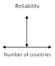
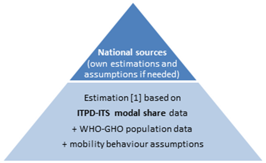
[1] E = Population * MD * BMS * BTL      

E=Exposure, i.e. km travelled by bicycle per year

Population: WHO data

MD= Mobility demand (3 all-mode trips per day, assumption)

BMS=Bicycle modal share, i.e. bicycle trips per total trips (ITDP-ITS extrapolations by world region)

BTL= Bicycle trip length (3 km per bicycle trip, assumption)

ITDP-ITS = Institute for Transportation and Development Policy and Institute of Transportation Studies

WHO-GHO = WHO Global Health Observatory

The above-mentioned sources are of different quality, and combining them implies different levels of reliability of the resulting fatality risk estimates. Five levels of reliability were considered based on the data quality of the datasets used for fatalities (numerator of the fatality risk estimate) and exposure (denominator).

·       very high: numerator from International Transport Forum fatality data and denominator from national sources;

·       high: numerator from International Transport Forum fatality data and denominator from national sources that imply some calculations or assumptions;

·       medium: numerator from International Transport Forum fatality data and denominator estimated based on modal share extrapolation by the Institute for Transportation and Development Policy;

·       low: numerator from observed WHO Global Health Observatory fatality data and denominator estimated based on modal share extrapolation by the Institute for Transportation and Development Policy; and

·       very low: numerator from modelled WHO Global Health Observatory fatality data and denominator estimated based on modal share extrapolation by the Institute for Transportation and Development Policy.

Back to homepage         Back to how HEAT works            Back to crash risk assessment

Sources

1.        Development of the Health economic assessment tools (HEAT) for walking and cycling. Consensus meeting. Copenhagen, Denmark, 28-29 March 2017. Meeting background document. Copenhagen: WHO Regional Office for Europe, 2017.

2.        Teschke K, Harris MA, Reynolds CCO, Winters M, Babul S, Chipman M, et al. Route infrastructure and the risk of injuries to bicyclists: a case-crossover study. Am J Public Health. 2012 Dec;102(12):2336–43

3.        Jacobsen PL. Safety in numbers: more walkers and bicyclists, safer walking and bicycling. Inj Prev. 2003 Sep 1;9(3):205–9

4.        Elvik R. The non-linearity of risk and the promotion of environmentally sustainable transport. Accid Anal Prev. 2009 Jul;41(4):849–55

5.        Schepers JP, Heinen E. How does a modal shift from short car trips to cycling affect road safety? Accid Anal Prev. 2013 Jan;50:1118–27

6.        Development of the Health economic assessment tools (HEAT) for walking and cycling (PASTA – WP4). Core group meeting. Copenhagen, Denmark, 2-3 November 2016. Meeting report. Copenhagen: WHO Regional Office for Europe, 2017.

7.        ITF-IRTAD International Transport Forum – International Traffic Safety Data and Analysis Group. Database Casualties by age and road use. 2017. Online database. http://stats.oecd.org/Index.aspx?DataSetCode=IRTAD_CASUAL_BY_AGE

8.        WHO-GHO World Health Organisation - Global Health Observatory data repository. 2016. Online data base. http://apps.who.int/gho/data/node.main.A997?lang=en

9.        ITDP-ITS. Institute for Transportation & Development Policy and the University of California. A Global High Shift Cycling Scenario: The Potential for Dramatically Increasing Bicycle and E-bike Use in Cities Around the World, with Estimated Energy, CO2, and Cost Impacts. 2015. https://www.itdp.org/wp-content/uploads/2015/11/A-Global-High-Shift-Cycling-Scenario_Nov-2015.pdf

10.     Diaz Olvera L, Plat D, Pochet P. The puzzle of mobility and access to the city in Sub-Saharan Africa. J Transp Geogr. 2013 Oct;32:56–64

11.     WALCYNG. How to enhance WALking and CYcliNG instead of shorter car trips and to make these modes safer (Deliverable D6) [Internet]. 1997. Available from: https://safety.fhwa.dot.gov/ped_bike/docs/walcyng.pdf

Carbon assessment in HEAT – overview

The carbon emissions in HEAT consists of three main assessment steps¹:

1.      Assessing true mode shift from motorized travel to walking or cycling (or vice-versa);

2.      Assessing the carbon emissions from substituted motorized travel; and

3.      Assessing the economic value of the social impact of changes in carbon emissions.

HEAT can assess the modal shift from motorized travel in assessments that compare two cases (for example, reference versus comparison, before versus after an intervention and with policy measures versus without policy measures). After entering a volume of walking and/ or cycling, users are asked to adjust their data to consider the shares of walking and/or cycling that:

·                      have been reassigned (shifted from other routes or destinations) or are entirely new because of induced (or generated) demand, both of which are not considered for the carbon assessment; for example, if 5% of new cycling was a shift from a parallel route and 5% was newly induced travel, the cycling activity relevant to the carbon assessment is 90% of the volume initially entered by the user.

·       are mainly for transport (versus for recreation); assuming that any walking and/or cycling for recreation will not have been shifted from or carried out by motorized travel, the carbon assessment does not consider the volume of recreational active travel.

·       were shifted from other motorized modes. For these modal shifts, changeable default diversion rates are provided (see diversion rates).

Single-case assessments (which assumes a steady-state situation), by definition exclude reassigned and induced walking and/or cycling. In this case, the proportions shifted from other modes are used to derive the amount of motorized travel that hypothetical would have been carried out otherwise (for no walking and/or cycling). The same approach applies to two-case assessment in which the user has selected the option of “no data” on motorized modes (input data section).

The second step converts the above changes in travel activity into carbon emissions that are potentially avoided (single case assessment) or saved (two case assessments). For this calculation step, the HEAT approach includes:

·       operational emissions  
(including country- and year-specific background values on average trip lengths, fuel splits, vehicle fleet compositions , ambient temperature, ‘cold start’ excess emissions  and a changeable default value on prevailing traffic conditions in the study area);

·       energy supply emissions
(including country- and year-specific background values on “well-to-tank” emissions for different transport fuels such as gasoline, diesel, and electricity); and

·       vehicle lifecycle emissions
(using a standard lifecycle inventory approach applying embedded carbon emissions factors for materials and energy used in vehicle manufacturing).  

In the third step, the resulting saved carbon emissions are monetized using the “Social Cost of Carbon” (SCC) approach (more information see here.) Changeable default values are provided disaggregated by country and start year of economic assessment.

Back to homepage         Back to how HEAT works            Back to how HEAT assessments work

Sources

1.        Development of the health economic assessment tools (HEAT) for walking and cycling. 5^th Consensus meeting. Meeting report. Copenhagen, Denmark, 28 - 29 March 2017. Copenhagen: WHO Regional Office for Europe; 2017.

Carbon module: guidance on “mode shift” and “diversion rates” (step 1)

What are diversion rates? How is mode shift handled in the carbon module?

The carbon tool excludes new trips that do not displace trips made previously by motorized modes from the assessment of carbon emissions from motorized travel. This has been implemented by parameterizing diversion rates [1] for walking and cycling for transport, with values between 0 and 100% for the shares of new cycling (or walking) estimated to be shifted from motorized travel and walking (or cycling). The motorized modes considered include cars (as driver or passenger), local buses, urban rail (including tram and underground) and motorcycles (not shown separately in Figure 1 for space reasons). For two-case assessment, the user is asked to consider excluding any induced (entirely new trips not replacing motorized travel) or reassigned (route shift) travel activity. The diversion rates are applied to the volume of walking and/or cycling entered by the user.

Figure 1: HEAT assessment of carbon emissions: modal shift using travel activity and diversion rates

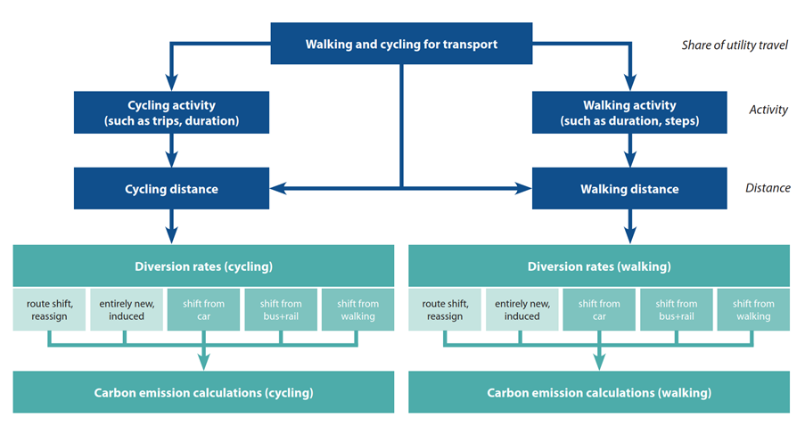
Note: the dashed boxes are only really relevant for assessments of ‘before’ vs. ‘after’ comparisons.

An example

Assume an infrastructure intervention has led to an increase in connectivity, making it easier and safer to travel via the new route. New cycling trips are being recorded along that route (such as by using trip counters or user intercept surveys). Some of the new trips were made previously using different modes (modal shift), and some were on a parallel route that perhaps was not as convenient or safe to use (route shift or route reassignment). Some even did not exist at all before the intervention (newly generated or induced demand that was suppressed before). The carbon module focuses on the former (modal shift) and does not consider the latter (route shift and newly induced trips).

Changeable default values

For the diversion rates of the remaining volume of walking or cycling, HEAT provides recommended values based on a conservative assessment of the evidence found in the appraisal guidance [2-5] and impact scenario [6-8] literatures. For instance, UK transport appraisal guidance (WebTAG) [1] and Mulley et al [9] reported car substitution rates of 25% to 30%. ECF [10] suggested to use: car 32%, bus 42% and walking 26%, based on mode substitution rates observed for bicycle trips of bicycle share schemes.

Table 1 shows the HEAT-recommended default values for diversion rates from other transport modes to cycling or walking.

Table 1: changeable default values for mode shift / diversion rates

Back to homepage         Back to how HEAT works            Back to carbon assessment

Sources

1.              DfT. Transport analysis guidance: WebTAG, https://www.gov.uk/guidance/transport-analysis-guidance-webtag. 2014.

2.              Dons, E., et al., Physical Activity through Sustainable Transport Approaches (PASTA): protocol for a multi-centre, longitudinal study. BMC Public Health, 2015. 15: p. 1126.

3.              Brand, C., A. Goodman, and D. Ogilvie, Evaluating the impacts of new walking and cycling infrastructure on carbon dioxide emissions from motorized travel: A controlled longitudinal study. Applied Energy, 2014. 128(0): p. 284-295.

4.              Goodman, A., S. Sahlqvist, and D. Ogilvie, Do new walking and cycling routes increase physical activity? One- and two-year findings from the UK iConnect study. Am J Public Health, 2014. 104.

5.              European Commission, OBIS (Optimising Bike Sharing in European Cities), Final Report. 2011, Brussels: European Commission.

6.              Woodcock, J., et al., Public health benefits of strategies to reduce greenhouse-gas emissions: urban land transport. The Lancet, 2009. 374.

7.              Keogh-Brown, M., et al., A whole-economy model of the health co-benefits of strategies to reduce greenhouse gas emissions in the UK. The Lancet, 2012. 380, Supplement 3(0): p. S52.

8.              Buekers, J., et al., Health impact model for modal shift from car use to cycling or walking in Flanders: application to two bicycle highways. Journal of Transport & Health, 2015. 2(4): p. 549-562.

9.              Mulley, C., et al., Valuing active travel: Including the health benefits of sustainable transport in transportation appraisal frameworks. Research in Transportation Business & Management, 2013. 7(0): p. 27-34.

10.            ECF, Cycle more Often 2 cool down the planet! - Quantifying CO2 savings of Cycling. 2011, European Cyclists' Federation (ECF): Brussels.

Carbon assessment in HEAT: Carbon emissions (step 2)

Operational emissions

Operational carbon emissions are derived by breaking carbon emissions down into changes in travel demand (passenger-km, by mode – see step 1, differences in energy efficiency (megajoules per passenger-km, by mode and fuel type) and differences in carbon intensity (CO2e/MJ, by mode and fuel type); (that is, a typical decomposition approach):

Figure: Composition of operational carbon emissions

HEAT considers the effects of three contextual factors on carbon emission factors:

1.      distance and average trip lengths;

2.      average speed, representing various traffic conditions in the study area; and

3.      mode characteristics such as vehicle type and fuel type.

For cars, HEAT considers average traffic speeds, vehicle fleet composition and the effect of real-world driving (adding 21.6% to the carbon emissions derived from official laboratory test data; value based on the conversion factors used in the United Kingdom [1]) in the study area to calculate the “hot” emission of CO2e emitted per km, based on published relationships between fuel consumption, average speed and conversion to carbon emissions using a standard carbon balance method. For motorcycle, bus and rail, only fuel type shares are considered, with average emission factors based on the conversion factors used in the United Kingdom [1]. Buses are mainly powered by diesel power trains; motorcycles are 100% gasoline; and urban rail is assumed to be all electric. For cars, cold-start excess emissions (for the cold driving for each trip, typically the first 3.4 km after starting) are added to this. This can be specified as follows::

Where: E_t=pollutant emissions (e.g. CO₂e); t=scenario (e.g. “without” and “with” intervention), ef_hot,t(mode)=“hot” emissions factor for mode in scenario t; pkm_t(mode)=passenger-km for mode in scenario t, E_cold=cold start excess emissions (for cars only); temp=ambient temperature; trip length=average trip length.

The first term includes speed-dependency of emissions factors as follows (based on the European Environment Agency’s COPERT model [2]):

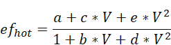
Where: V=average speed and coefficients a to e are empirically derived for each fuel and hard coded in the HEAT module.

Hot emissions dominate total emissions, but cold-start emissions should not be neglected, since they constitute a significant share of total emissions for shorter trip lengths (typically 15–20%). Ecold is typically derived for each vehicle technology k as:

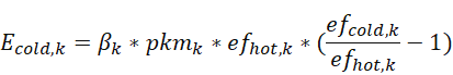
Where: b = fraction of mileage driven with a cold engine or the catalyst operated below the light-off temperature, pkm_k = passenger-km, e_cold / e_hot = cold/hot emission quotient for vehicles of technology k, temp=ambient temperature. l = 1.47, m=0.009 (gasoline); l=1.34, m=0.008 (diesel) based on [2]

The b parameter depends upon ambient temperature and average trip length (see [2] for details). In HEAT, b was derived by dividing average trip length of the substituted car trip by an average cold start distance of 3.4 km, with b <= 1.

Vehicle fuel type shares and average occupancy rates are based on international databases, including the GAINS (greenhouse gas–air pollution interactions and synergies) model projections (scenario WPE_2014_CLE of the Council Working Party on Environment (WPE) based on current legislation (CLE)) of the International Institute for Applied Systems Analysis for years up to 2050 [3-7]. Future projections of carbon emissions factors are thus based on available scenario data, not forecasts, therefore any projections beyond the 10-year timeframe should be treated with caution.

For cars, the user can choose between five generic traffic conditions based on typical road speeds observed in the European countries, including: Vienna 46 km/h, Newcastle 42 km/h (i.e. “nearly free flow conditions”); Prague 37 km/h, Barcelona 35 km/h, Paris 31 km/h, Edinburgh 30 km/h, Rome 30 km/h (“some heavy traffic and peak time congestion”); and London 19 km/h, Brussels 22 km/h (“heavy congestion and wider peaks”) [8, 9]. The five categories are:

·       European average, urban (32 km/h) – changeable default value;

·       Little or no congestion, urban (“free flow”) (45 km/h);

·       Some peak time congestion (commute, school run), urban (35 km/h);

·       Heavy congestion most days (am, pm and inter peak), urban (20 km/h);

·       European average, rural (60 km/h).

HEAT uses country and year specific emissions factors. Table 1 provides an example for the United Kingdom in 2015.

Table 1: Derived average hot and cold emission factors (tailpipe, tank-to-wheel), showing values derived for the United Kingdom in 2015 (HEAT uses country- and year-specific factors)

Notes: ⁽¹⁾ Takes into account weighted fuel/engine type shares for each mode, e.g. for cars in the UK in 2015 (56% petrol, 43% diesel, 1% electric), bus (100% diesel), motorcycle (100% gasoline). ⁽²⁾ Car occupancy rate of 1.56 (all trip purposes), 12.21 (local buses), 40 (average urban rail/tam/metro), 1.05 (average motorcycle). ⁽³⁾ With cold/hot ratio of 1.33 and cold trip distance of 3.51 km, derived from ambient temperature of 9.4 degrees C and average trip length of 14 km.
n.a. = not applicable.

Sources: hot and cold emissions factor coefficients [2, 10]; vehicle fleets [1, 3, 11, 12].

Back to homepage         Back to how HEAT works            Back to carbon assessment

Sources

1.              DEFRA/DECC, UK Government conversion factors for Company Reporting, full 2016 dataset. 2016, Department for the Environment, Food and Rural Affairs and Department for Energy and Climate Change: London.

2.              EEA, COPERT IV. 2012, European Environment Agency: Copenhagen.

3.              ACEA/ANFAC, European Motor Vehicle Parc 2014: Vehicles in Use (2009-2014). 2014, Madrid: ANFAC/ACEA.

4.              SMMT, New Car CO₂ Report 2014: The 13th report. 2014, London: The Society of Motor Manufacturers and Traders (SMMT).

5.              IEA, World energy outlook 2015. 2015, Paris: International Energy Agency (IEA).

6.              Eurostat, Transport data database, October 2015 update. Last accessed at http://ec.europa.eu/eurostat/web/transport/data/database on 10/03/2017. 2016, Brussels: Eurostat, European Commission.

7.              IIASA, IIASA GAINS model, scenario WPE_2014_CLE: the updated ‘current legislation’ (after the bilateral consultations in 2014) of the PRIMES 2013 REFERENCE activity projection. 2014, IIASA: Laxenburg, Austria.

8.              Olson, P. and K. Nolan, In Depth: Europe's Most Congested Cities, last accessed at https://www.forbes.com/2008/04/21/europe-commute-congestion-forbeslife-cx_po_0421congestion_slide.html on 10/02/2017. Based on INRIX data., in Forbes. 2008.

9.              Newman, P. and J. Kenworthy, Sustainability and Cities: Overcoming Automobile Dependence. 1999, Washington, DC: Island Press.

10.            EMEP/EEA, EMEP/EEA air pollutant emission inventory guidebook 2016, Technical guidance to prepare national emission inventories. 2016, European Environment Agency: Copenhagen.

11.            SMMT, UK new car market starts 2016 on a high with best January in 11 years, http://www.smmt.co.uk/2016/02/uk-new-car-market-starts-2016-on-a-high-with-best-january-in-11-years/ [last accessed on 18/01/2016]. 2016, SMMT: London.

12.            DfT, Transport Statistics Great Britain: 2015 Edition. 2015, Department for Transport: London.

HEAT carbon assessment: carbon emissions (step 2)

Energy Supply Emissions

Carbon emissions from energy supply include upstream emissions from the extraction, production, generation and distribution of energy supply. The adopted approach uses well-to-tank emission factors for various energy supply pathways for transport fuels (gasoline, diesel, electricity, etc.) [1], taken from published and well respected sources including the JEC Well-to-Wheels study [2] and its use in developing national recommended values such as the United Kingdom Department for the Environment, Food and Rural Affairs and Department for Energy and Climate Change [3]. For E-bikes, cars, buses and urban rail, this is based on different values for the JEC well-to-wheels study of gasoline (0.654 kg of CO2e per kg of fuel), diesel (0.688 kg of CO2e per kg of fuel) and delivered electricity (for example, this was 0.517 kg of CO2e for the United Kingdom in 2015). As with operational emissions, an additional 21.6% was added to account for real-world driving conditions. Since electricity factors vary significantly between countries (up to three orders of magnitude, reflecting the use of high shares of renewable sources versus high shares of fossil fuels), HEAT uses country-specific factors based on the widest possible country comparison from an authoritative source [4].

Table 1 provides an example for the United Kingdom in 2015.

Table 1: Derived average energy supply emissions factors (well-to-tank) per passenger-km, showing values derived for the United Kingdom in 2015 (HEAT uses country- and year-specific factors)

Notes: ⁽¹⁾ weighted by fuel/engine type shares for each mode, e.g. for cars in the UK in 2015 (56% petrol, 43% diesel, 1% electric), bus (100% diesel), motorcycle (100% gasoline). ⁽²⁾ Car occupancy rate of 1.56 (all trip purposes), 12.21 (local buses), 40 (average urban rail/tam/metro), 1.05 (average motorcycle). n.a. = not applicable

Main sources: well-to-tank emissions factors [2, 3]; electricity emissions factors [4]; vehicle fuel shares [5].

Back to homepage         Back to how HEAT works            Back to carbon assessment

Sources

1.               Odeh, N., N. Hill, and D. Forster, Current and Future Lifecycle Emissions of Key „Low Carbon‟ Technologies and Alternatives, Final Report. 2013, Harwell, UK: Ricardo AEA for the Committee on Climate Change.

2.               JEC, JEC Well-To-Wheels Analysis, Report EUR 26237 EN - 2014. Last accessed at http://iet.jrc.ec.europa.eu/about-jec/sites/iet.jrc.ec.europa.eu.about-jec/files/documents/report_2014/wtt_report_v4a.pdf on 10/03/2017. 2014, Brussels: JEC - Joint Research Centre-EUCAR-CONCAWE collaboration.

3.               DEFRA/DECC, UK Government conversion factors for Company Reporting, full 2016 dataset. 2016, Department for the Environment, Food and Rural Affairs and Department for Energy and Climate Change: London.

4.               Ecometrica, Electricity-specific emission factors for grid electricity. 2011: Ecometrica.

5.               IIASA, IIASA GAINS model, scenario WPE_2014_CLE: the updated ‘current legislation’ (after the bilateral consultations in 2014) of the PRIMES 2013 REFERENCE activity projection. 2014, IIASA: Laxenburg, Austria.

HEAT carbon assessment: carbon emissions (step 2)

Vehicle lifecycle emissions

HEAT considers lifecycle carbon emissions from the manufacture of vehicles (the clear majority of vehicle life-cycle carbon emissions, apart from operational ones), with aggregate carbon values per vehicle type (cars, motorcycles, bikes and public transport vehicles) derived assuming typical lifetime mileages, mass body weights, material decomposition and material-specific emission and energy use factors.

The key inputs, assumptions and derived carbon emissions factors per passenger-km are shown for India in Table 1. The HEAT tool uses time independent but country-specific factors, reflecting local differences in occupancy rates for the different motorized modes [1].

Table 1: Assumptions and average CO₂e emissions from vehicle manufacture

^($) battery and motor add 7kg in weight; assumed 2.5 gCO₂e/km for the battery based on [2]. ^(*) Car occupancy rate of 1.5 (all trip purposes), local bus 14.3, average urban rail 120, motorcycle 1.05.

Sources: lifecycle data [2]; electricity emissions factors [3]; vehicle fuel shares [4]; load factors [1].

Back to homepage            Back to how HEAT works                 Back to carbon assessment

Sources

1.              EC DG Climate Action, Transport database TRACCS (Transport data collection supporting the quantitative analysis of measures relating to transport and climate change). 2013, Brussels: Emisia, Infras and IVL for the European Commission.

2.              Odeh, N., N. Hill, and D. Forster, Current and Future Lifecycle Emissions of Key „Low Carbon‟ Technologies and Alternatives, Final Report. 2013, Harwell, UK: Ricardo AEA for the Committee on Climate Change.

3.              Ecometrica, Electricity-specific emission factors for grid electricity. 2011: Ecometrica.

4.              IIASA, IIASA GAINS model, scenario '6DS' for IEA World Energy Outlook, available for Europe (for 48 countries), Asia, with separate implementations for China (31 provinces and India (15 States), and for Annex I countries of the UNFCCC Convention. Accessed at https://gains.iiasa.ac.at/models/gains_models3.html in July 2019. 2016, IIASA: Laxenburg, Austria.

Default and background values for the HEAT calculations

Back to homepage         Back to how HEAT works            Back to data needs

Wherever possible, the HEAT provides generic data which are based on best available evidence or expert judgement. There are two types of generic values in HEAT:

1.      default values that are provided for a HEAT assessment but that can be overwritten by the users if they prefer to use other values, e.g. from their specific local context.

2.      background values  considered to represent the best possible scientific consensus (e.g. estimates based on numerous epidemiological studies) that cannot be changed by the user.

Below, an overview of the main default and background values is provided, with their source, used either for general calculations (e.g. to derive volume data for the calculations) or in the different HEAT modules.

Default values

General values

* This means a decision taken by the HEAT advisory group based on expert judgement

In addition, default values are provided (per country) for the mortality rates (7), values of statistical life (8) and social costs of carbon (9,10). 

Physical activity

The HEAT physical activity module uses only non-changeable background values, see next section.

Air pollution

The HEAT air pollution module provides default PM2.5 concentrations by country and cities as available from the WHO Global Health Observatory Repository (11).

Crashes

Besides that, the HEAT crashes module uses only non-changeable background values, see next section.

Carbon

Background values

General value

Physical activity

Air pollution

Crashes

For the HEAT crash assessment, background crash rates (per country and for future editions, per city,) are being used. For more information, see here (21).

Carbon

Back to homepage         Back to how HEAT works            Back to data needs

Sources:

1. Diaz Olvera et al. The puzzle of mobility and access to the city in Sub-Saharan Africa. Journal of Transport Geography Volume 32, October 2013, Pages 56-64 (http://www.sciencedirect.com/science/article/pii/S0966692313001634).

2. WALCYNG. How to enhance WALking and CYcliNG instead of shorter car trips and to make these modes safer (Deliverable D6) [Internet]. 1997. Available from: https://safety.fhwa.dot.gov/ped_bike/docs/walcyng.pdf

3. Kelly P et al. Systematic review and meta-analysis of reduction in all-cause mortality from walking and cycling and shape of dose response relationship. International Journal of Behavioral Nutrition and Physical Activity. 2014, 11:132  doi:10.1186/s12966-014-0132-x.)

4. Department for Transport. National Travel Survey [website] (national travel survey of England and Wales 2010-2014). https://www.gov.uk/government/collections/national-travel-survey-statistics. Published 2013, last updated 2017.  

5. Statistics Netherlands. OViN (Onderzoek Verplaatsingen in Nederland). 2013-14: Statistics Netherlands, The Hague/Heerlen/Bonaire.

6.  Kahlmeier S et al.  Health economic assessment tools (HEAT) for cycling and walking. Methodology and user guide. Copenhagen: WHO Regional Office for Europe; 2011.

7. World Health Organization Regional Office for Europe. European Detailed Mortality Database. 2015 (http://data.euro.who.int/dmdb/)

8. Mortality risk valuation in environment, health, and transport policies. Paris: OECD; 2012   (http://www.oecd.org/environment/mortalityriskvaluationinenvironmenthealthandtransportpolicies.htm, accessed 26 March 2014).

9. International Transport Forum (ITF), Adapting Transport Policy to Climate Change: Carbon Valuation, Risk and Uncertainty. 2015: OECD Publishing.

10. Smith, S. and N.A. Braathen, Monetary Carbon Values in Policy Appraisal, available at: http://www.oecd-ilibrary.org/content/workingpaper/5jrs8st3ngvh-en. OECD Environment Working Papers. 2015, Paris: Organisation for Economic Co-operation and Development.

11. World Health Organization. WHO Global Health Observatory (GHO) data [website]. (http://www.who.int/gho/en/) 2017.

12. Department for Transport. Transport analysis guidance: WebTAG, https://www.gov.uk/guidance/transport-analysis-guidance-webtag. 2014.

13. ECF, Cycle more Often 2 cool down the planet! - Quantifying CO2 savings of Cycling. 2011, European Cyclists' Federation (ECF): Brussels.

14. European Commission, OBIS (Optimising Bike Sharing in European Cities), Final Report. 2011, Brussels: European Commission.

15. Kahlmeier S, Götschi T, Cavill N, Fernandez AC, Brand C, Rueda DR et al. Health economic assessment tool (HEAT) for cycling and walking. Methods and user guide on physical activity, air pollution, injuries and carbon impact assessments. Copenhagen: WHO Regional Office for Europe; 2017

16. Development of the Health Economic Assessment Tools (HEAT) for walking and cycling. 4^th Consensus meeting: meeting background document. Bonn, 11-12 December 2014. Copenhagen, WHO Regional Office for Europe, 2014.

17. WHO expert meeting: methods and tools for assessing the health risks of air pollution at local, national and international level. Meeting report, Bonn, Germany, 12–13 May 2014. Copenhagen: WHO Regional Office for Europe; 2014 (http://www.euro.who.int/en/health-topics/environment-and-health/air-quality/publications/2014/who-expert-meeting-methods-and-tools-for-assessing-the-health-risks-of-air-pollution-at-local,-national-and-international-level, accessed 26 June 2015).

18. De Nazelle et al. Comparison of air pollution exposures in active vs. passive travel modes in European cities: A quantitative review. Environment International 2017 (99): 151-160 (Appendix C). (http://www.sciencedirect.com/science/article/pii/S0160412016304585?via%3Dihub, accessed 31 August 2017).

19. Johnson T (2002): A guide to selected algorithms, distributions, and databases used in exposure models developed by the office of air quality planning and standards. US Environmental Protection Agency.

20. de Nazelle A, Rodríguez DA, Crawford-Brown D (2009): The built environment and health: impacts of pedestrian-friendly designs on air pollution exposure. The Science of the total environment 407(8):2525-35

21. Health economic assessment tool (HEAT) for cycling and walking. Copenhagen: WHO Regional Office for Europe; 2011; revised edition published online 2017 (www.heatwalkingcycling.org).

22. DfT. Average speed and delay on local “A” roads. 2015, Department for Transport: London.

23. Free flow vehicle speeds in Great Britain: 2015 [website]. London: Department for Transport (https://www.gov.uk/government/statistics/free-flow-vehicle-speeds-in-great-britain-2015)

24. Statista:  Average speed in Europe's 15 most congested cities in 2008 (in kilometers per hour) (available at https://www.statista.com/statistics/264703/average-speed-in-europes-15-most-congested-cities/) (no year).

25. DfT. Transport Statistics Great Britain. 2016, Department for Transport: London.

26. Leuenberger M, Frischknecht R. (2010) Life Cycle Assessment of Two Wheel Vehicles. Uster: ESU-services

27. del Duce, A. Life Cycle Assessment of conventional and electric bicycles. Paper presented at Eurobike (31 August - 3 September 2011), 2011: Friedrichshafen, Germany.

28. Ricardo AEA. Current and Future Lifecycle Emissions of Key “Low Carbon” Technologies and Alternatives, Final Report. 2013, Ricardo AEA for the Committee on Climate Change: Harwell, UK.

29. DfT. National Travel Survey: the way we travel. 2015, Department for Transport: London

Monetization of the HEAT results

HEAT also allows calculating an economic value of the mortality and carbon effects. To monetize the effects on mortality, the “Value of statistical Life” (VSL) is used.

For the carbon effect, a methodology based on the “Social Costs of Carbon” (SCC) is used.

The results can also be discounted to consider that economic benefits occurring in the future are generally considered less “valuable” than benefits occurring in the present. The lower the discount rate the higher the user weighs future economic benefits in the overall assessment.

As default value, a discount rate of 5% has been set.

If the results of economic appraisal with HEAT will be included as one component into a more comprehensive cost-benefit analysis of transport interventions or infrastructure projects, the final result of the comprehensive assessment would then be discounted to allow the calculation of the present value. In this case, enter "0" here.

Back to homepage         Back to how HEAT works            Back to default and background values

Value of statistical life

What is the value of a statistical life?

The value of a statistical life (VSL) is derived using a method called willingness to pay. It aggregates individuals’ willingness to pay to secure a marginal reduction in the risk of premature death in relation to the years this person can expect to live according to the statistical life expectancy.

According to economic theory, the willingness to pay captures perceptions of risks and potential costs borne by the individual person rather than society, including lost consumption, immaterial costs (such as suffering) and the share of health costs paid directly by the victims. Thus, it should account for multiple domains, including consumption, inability to work, the health-care costs the individual pays (and not insurers) and their own pain and suffering. Thus, it represents the societal economic value of reduced premature mortality and is often used in transport appraisal.

The VSL is not the value of an identified person’s life but rather an aggregation of individual values for small changes in risk of death: for example, how much a representative sample of the population would be willing to pay (in monetary terms) for a policy that would reduce their annual risk of prematurely dying from 3 in 10 000 to 2 in 10 000.

Approach to calculating the default values for HEAT

The default values were calculated based on a comprehensive review of VSL studies by the OECD (1): Studies were only included if they were based on a representative population sample of at least 200 subjects and provided information on the size of the risk change in question. A total of 261 values from 28 studies were selected to calculate the base VSL for adults in OECD countries of US$ 3.0 million, with a range from US$ 1.5 million to US$ 4.5 million (in 2005 US dollars). The international advisory group concluded that the OECD report represented the best currently available evidence.

The following formula was applied to derive the country-specific values in local currency for the year 2015, applying adjustments to account for income differences across countries, inflation and income growth over time and conversion of the currency from US dollars to local currency using exchange rates adjusted for purchasing power parity (PPP).

VSL _{COUNTRY, 2015 (local currency)} = VSL_{OECD, 2005, USD} * (Y_{COUNTRY, 2005} / Y_OECD, 2005) ^0.8 * PPP₂₀₀₅ 
* (1 + % Δ P_2005-2015 ) * (1 +% Δ Y_2005-2015 )^0.8

VSL_{OECD, 2005, USD} = base value for OECD of 3.013 million US$ from OECD-study (±50%) (1)

Y_{COUNTRY, 2005} = real GDP per capita at purchasing power parity in 2005 of the respective country (2)

Y_{OECD, 2005} = average real GDP per capita at purchasing power parity in 2005 of OECD-countries, which equals 30’801 (US$ in 2005) (2)

0.8 = income elasticity of VSL according to the OECD-study (1)

PPP₂₀₀₅ = Purchasing power parity-adjusted exchange rate in 2005 (local currency / US$) (2)

(1 + %ΔP _2005-2015 ) = inflation adjustment with consumer price index of the respective country between 2005 and 2015

(1 +% Δ Y_2005-2015 ) = income adjustment with growth in real GDP per capita in the respective country between 2005 and 2015

Using exchange rates, the country-specific values in local currencies were also transformed into euros. With these euro values and using the population-weighted averages of the country-specific VSL, average values for the average values for the 27 EU countries from 2007 to 2013 (EU27), the 28 current EU countries including Croatia (EU28) and the 53 countries of the WHO European Region were calculated for 2015 (only available for 2005 for Azerbaijan, Belarus and Tajikistan and based on the values for other countries for six more countries)*.

The European default values (for 2015) of €2.132 million (WHO European Region), €2.891 million (EU27 countries) or €2.877 million (EU28 countries including Croatia) can also be used.

Figure 1 European average values for VSL based on different definitions of the region

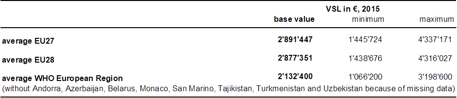
Back to homepage         Back to how HEAT works            Back to default and background values

Sources

1.        Mortality risk valuation in environment, health, and transport policies. Paris: OECD; 2012.

2.        World Bank Search (database). Paris, World Bank Group, 2014 (http://search.worldbank.org/data, accessed 4 September 2017)

*       No national default VSL could be derived for nine countries. For Andorra, the value for Spain is used as default; for Liechtenstein, Switzerland; for Monaco, France; and for San Marino, Italy. For Turkmenistan, the value is based on data for Georgia, and for Uzbekistan, Kyrgyzstan. The values for 2005 (based on approximations using countries with the most similar GDP per capita level in the vicinity) are shown as default values for Azerbaijan (using data for Georgia), Belarus (using data for the Russian Federation) and Tajikistan (using data for Kyrgyzstan)

Carbon emissions (step 3)

Social Cost of Carbon

The social costs of carbon can be defined as the monetized value of the global damage caused by the incremental impact of an additional tonne of carbon dioxide equivalent (CO2e) emitted at a specific point in time.

Carbon values based on the social costs of carbon method essentially put a price on carbon. The damage costs are estimated using integrated assessment models such as the Dynamic Integrated Climate-Economy model (DICE) (1,2), Climate Framework for Uncertainty, Negotiation and Distribution (FUND) (3) and Policy Analysis of the Greenhouse Effect (PAGE) model (4). The values of the social costs of carbon vary widely: for example, one meta-analysis of 211 estimates from 47 studies (5) found a wide distribution of carbon values, from –€1 to €451 per tonne of CO2e. Key issues in measuring the social costs of carbon are the extent of uncertainty in methods and data, time horizon, the use of discounting, geographical scope (such as global versus regional) and equity weighting. The carbon values used in policy assessment vary by country and increase over time.

The international advisory group agreed to use country-specific carbon values based on the social costs of carbon approach in HEAT, since this is used in project appraisal independently of national emission targets and mitigation policies (6).

Monetization of the carbon emissions

Changeable default values for the SCC are provided by country and year (Figure 1), based on international evidence, regional averages (6,7) or country specific values (if existing). The values for the social costs of carbon for countries or contexts not covered in existing evidence or policy guidance have been allocated to the European Commission recommended values: US$ 44 in 2015, rising to US$ 66 by 2030.

The users may override these and use their own recommended economic appraisal values instead.

Figure 1: Default carbon values by country and year of assessment (in USD/t CO₂e at 2015 values)

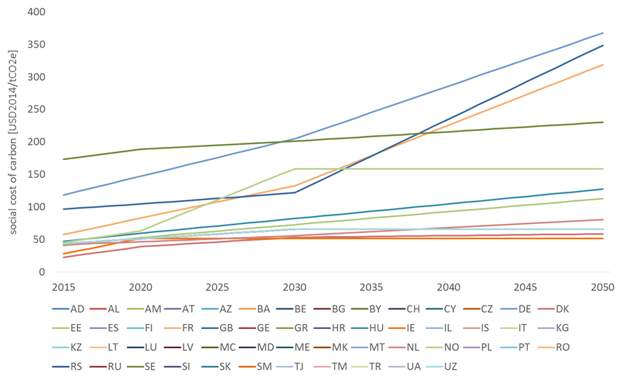
Back to homepage         Back to how HEAT works            Back carbon assessment              Back to economic valuation

Sources

1.        Moore FC, Diaz DB. Temperature impacts on economic growth warrant stringent mitigation policy. Nature Clim. Change, 2015. 5(2): p. 127-131.

2.        Nordhaus WD. Revisiting the social cost of carbon. Proceedings of the National Academy of Sciences, 2017. 114(7): p. 1518-1523.

3.        Anthoff, D. and R. S. J. Tol (2013) The uncertainty about the social cost of carbon: A decomposition analysis using FUND, Climatic Change 117(3): 515-530.

4.        Weisbach D, Moyer E. Discounting in Integrated Assessment. 2010, Washington D.C.: Resources for the Future.

5.        Tol RSJ. The Social Cost of Carbon: Trends, Outliers and Catastrophes. Economics: The Open-Access, Open Assessment E-Journal, 2008. 2: p. 2008-2025.

6.        ITF, Adapting Transport Policy to Climate Change: Carbon Valuation, Risk and Uncertainty. 2015: OECD Publishing.

7.        Smith, S. and N.A. Braathen, Monetary Carbon Values in Policy Appraisal, available at: http://www.oecd-ilibrary.org/content/workingpaper/5jrs8st3ngvh-en. OECD Environment Working Papers. 2015, Paris: Organisation for Economic Co-operation and Development.

Interpretation of the HEAT results

The HEAT results are shown in two steps:

·       the results summary, summing up the health and economic benefits and negative effects as well as carbon emission effects across all selected pathways (as selected by the user), as well as a brief summary of the data inputs made; and

·       the detailed results per mode (walking and/or cycling) and pathway (physical activity, air pollution, road crashes and carbon, as selected by the user).

The results summary first displays the amount of walking or cycling the user has entered and the number of people in the assessed population.

The tool produces an overall estimate of the following outputs (summing up positive and negative effects across health-related pathways and of reductions in carbon emissions, as selected by the user):

·       the number of premature deaths prevented (per year and across the full assessment period);

·       tonnes of emissions of CO₂ equivalents avoided (per year and across the full assessment period);

·       sum of the economic value of effects on mortality (from physical activity, air pollution and/or road crashes, as selected by the user; per year and across the full assessment period as well as discounted, if so selected), using VSL;

·       the economic value of the effects of carbon emissions (per year and across the full assessment period as well as discounted, if so selected), using the social costs of carbon; and

·       the total economic value of effects, summing up the economic benefits from the three health as well as carbon emission calculations, as selected by the user (per year and across the full assessment period as well as discounted, if so selected).

In an overview table, users can select the detailed results they want displayed (per mode (walking and/or cycling) and pathway (physical activity, air pollution, road crashes and carbon emissions). According to the selection made, the detailed results are then displayed for each of the selected modes and pathways, including the same information as the result summary described above.

The results are also available as overview graphs, with total results and with results per mode and per pathway.

Limitations and sensitivity analysis

Many of the variables used within this HEAT calculation are estimates and therefore liable to some degree of error. Remember that the HEAT tools provide you with an approximation of the level of health, carbon emission and economic benefits. Several assumptions apply. To get a better sense of the possible range of the results, you are strongly advised to rerun the model, entering slightly different values for variables for which you have provided a best guess, such as entering high and low estimates for such variables.

Back to homepage         Back to how HEAT works